Composing with Chaos: Applications of a New Science to Music

David Little

In this presentation, I will give an overview of the new chaos sciences, and show where they may be of application to composers with examples chosen from my own work.

Scientific and mathematical developments of the last 20 years have led to new insights into subjects which, because of their complexity, had previously been swept under the rug by the learned establishment. Intractable problems in weather forecasting, the modeling of wildlife populations, the geometry of nature, the studies of turbulent flow and bio-rhythms have all been recently revolutionized by new analytical methods. Concepts such as chaos, order, simple and complex have been redefined in relation to definitions of the fractal and fractal dimensionality. Comparable to the revolutions of Newton and Einstein, I believe that the new chaos sciences will have a substantial impact on society as a whole as these insights spread inevitably from mathematicians and scientists to economists, politicians and artists. Of course there may have been no direct connection between the classical style and Newton's laws of gravity or the post WWII composers's experimentations and Einstein's theory of relativity, but few doubt that artists draw profoundly on their cultural and intellectual backgrounds, and can therefore be regarded as mirrors of their times. Composers can also be catalysts for the future society; music-making can be a model for human interaction be it composers dictating to musicians or entering into co-operative bonds with them.

No less important than the avalanche of inventions and discoveries following from Newton's laws of motion is the belief at the philosophical level that the universe could be understood through logical thinking. This optimism was very well expressed already in the 18th century by the French astronomer Laplace. He stated that intelligent creatures could know any past or future state of the universe only if they knew well enough its present state, and what direction it was heading towards. This deterministic world view has proved to need revision however. The cracks in the wall appeared early in this century in the bizarre results from experiments with atomic particles which could only be "explained" through the extreme abstractions of Quantum Theory. Together with Relativity Theory, a world view emerged in which atomic particles are not small hard objects which can be observed impartially but probabalistic entities which may be in such-and-such a position however, like the very conditions of Time and Space themselves, subject to change via the presence of the observer. These insights, however shocking to the West, have been seen as astonishingly similar to the experiences of ancient Eastern mystics, the common denominator being the awareness of the unity and mutual interrelation of all things and events which are involved in ceaseless transformation.

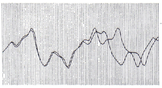
Ironically it has taken the advent of the deterministic tool par excellence, namely the computer, to force contemporary scientists to rethink the whole matter. With mathematical models, they have been able to make accurate predictions of planetary motions and tides for example. Everyone had thought that long-term weather prediction should also be possible; you just had to make much more calculations. In 1961, the meteorologist Edward Lorenz managed to model the earth's weather on a computer allowing one to monitor the recurrence of theoretical rain storms, or cyclones etc. but at a much faster speed. There was one problem however; if he started the program with slightly different initial conditions, of wind speed and temperature, the artificial weather would be the same as in a previous run only in the beginning. After a while, the weather would diverge from the previous run, and eventually end up completely different. To appreciate what this means, one must remember that the computer model was using proven physical laws of gas and water behavior and that it functioned in a completely deterministic manner with no additional input after it was started. With Lorenz dawned the idea that long-range forecasting was impossible. Small errors in measurement would multiply, cascading upwards in the scale of turbulence: from a puff of wind to continent-sized spirals. Lorenz called it the "Butterfly Effect" - theoretically, a butterfly stirring its wings in Peking could start a storm over New York the next month!

Figure 1: The Butterfly Effect

Lorenz later developed a more general mathematical model of fluid behavior. It describes the flow of heated fluid called convection. For example, when a pan of water is heated, the hotter water at the bottom tends to rise, because it is less dense. At the top of the pan it comes into contact with air which cools it off somewhat. Then the cooled denser water sinks back to the bottom of the pan. This circulation of fluid is called a convection cell, and remains smooth and orderly as long as the heat under the pan is moderate. However, if the heat is high, the water moves too fast to cool of very much; the convection cell breaks up and flow it is turbulent as portions of the water compete with each other to get to the top. Lorenz wrote an equation to model convection, using 3 variables in a non-linear relationship. (A linear relationship is where a change in one variable is mirrored by a proportional change in another variable: its graph is a straight line. A graph of a non-linear relationship, on the other hand, might show breaks, reversals, bends, etc.) The change in values of the variables with time can be traced out in what is called a phase diagram. (See Figure 2.) A point on the diagram represents the physical state of a system, actually in 3 dimensions. If a system heads toward a stable final state, its phase diagram would tend to localize to a point called the attractor. For a periodic system, the phase diagram would tend to be a closed loop of some kind. Lorenz's model proves to be aperiodic, with a kind of infinite complexity; it has a strange attractor! The trace of the model loops endlessly without repeating or crossing itself, flipping unpredictably from one side to the other. It does remain within bounds, however, and is not random: a pattern emerges resembling butterfly wings. Indeed, a new kind of order was discovered which was to reveal itself in analysis of many different natural phenomena; order within chaos. Lorenz's work started the revolution which was, like his "Butterfly Effect" to spread to many fields outside of meteorology.

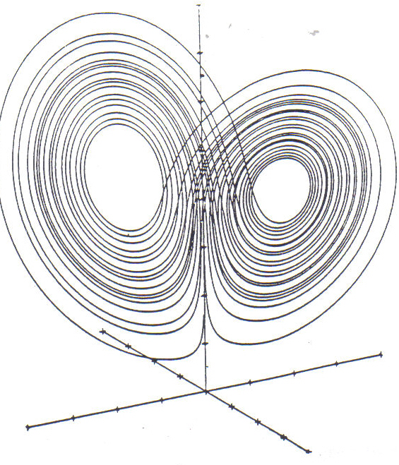
Figure 2: The Lorenz Function

At this point, I would like to present some of my own pieces which use some of the ideas just described. Harpsi-kord for tape and harpsichord was composed in 1988. In this piece the central idea is order within chaos. Compositionally, it swings between the polarities of regular vs. irregular, loud vs. soft, atonal vs. harmonic, and the use the timbre of an ancient instrument as opposed to an electronically generated timbre. A middle ground is sought in various transformations made possible through sampling techniques. Certain techniques were applied reflexively; having sampled a tone cluster, it was made available on each note of a synthesizer and clusters of clusters were made. Similarly rhythmic or melodic structures were nested in several layers at times. For example, one samples not a single tone, but a melodic motive, and loops it. By holding several keys with the same sample, one generates a polymetric texture, because the same loop at higher pitch plays faster, hence is shorter. One can sample this whole texture, and repeat the process, achieving very soon the limits of human perception of detail! The harpsichordist relates to the tape in a quasi-improvisational manner. Although the timing and pitch material is exactly notated, he/she is given considerable freedom in performance. For example, only the pitches were notated in a square with the rhythm and ordering improvised. (See Figure 3.) In this way another "feedback loop" is created; the improviser must use his/her ears and think fast in order to create a proper "dialogue " with the tape.

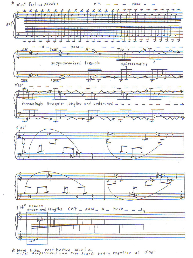
Figure 3: Harpsi-Kord, Pg.1

The next two pieces, Shuffle and Fractal Piano 6 (both from (1988) were realized with the help of the "Vorsetzer". The Vorsetzer is a new form of pianola developed by technicians of the Electronic Studio of the Sweelinck Conservatory, Amsterdam. It has 88 electromagnets which are mounted over the keys which can be triggered with varied degrees of force by a computer. The obvious advantage of this system over the old method of punching out rolls of paper is the inherent flexibility and compactness of data storage with computer. In addition, the use of the computer offers new compositional possibilities.

To make Shuffle, an 88-note chromatic scale was produced by, stored in and manipulated by computer. The scale accelerates smoothly from relative note values of quarters in the lowest register to 32nds in the highest. It has a dynamic curve of p<f>p with the loudest part occurring in the middle of the piano. MIDI-data for each note is stored in 3 separate memory allocations: for pitch, timing/length, and loudness. The data for some notes are then "shuffled" around a bit by a computer program which I devised: the contents of two randomly chosen (but nearby) memory units for pitch, for example, are exchanged. Likewise, length or loudness data for a few other different pairs are exchanged. The memory allocations are combined and read out to be "performed" by the Vorsetzer: one hears s slightly flawed chromatic scale. The memory allocations of the flawed scale are then subjected to the same process; data pairs are exchanged. Output is used for input for many cycles in a kind of feedback process. With each cycle, the scale becomes audibly more diffuse and irregular: notes migrate slowly away from their original position in the scale. The original perfectly ordered chromatic scale slowly "degenerates" into a "super-serial" shuffled mix. The final state is complex, and much dependent on the cumulative effect of many small random choices. In chaos theory, one would say that there is a sensitive dependence on initial conditions. As such, Shuffle is a musical model of the butterfly effect. Here it should be added that it also resembles a two voice cannon in contrary motion: a descending chromatic scale enters with the first "shuffled" version of the ascending scale, and receives similar treatment. (Sound example B.)

Fractal Piano 6 is one of a series of studies in which a computer program which I developed myself was used in combination with the Vorsetzer. The heart of the program is a model of population growth. The Malthusian Model describes the unbounded growth of a population (of fruit flies, for example) with x_n+1 = ax_n. This formula tells that we can find the population of a new generation x_n+1 by multiplying the number in the last generation x_n with the productivity factor, a. Suppose the population doubles each generation; then a=2, and starting with 2 parents, we'd get the series 4 children, 8 grandchildren, 16 great grandchildren, etc. Its easy to see that before many generations have been bred, we have a gigantic number. By the tenth generation, there would 1024 siblings.

In order to make a more realistic model, P.F. Verhulst in 1845 considered that in nature, the larger a population grows, the less productive it becomes; or the more the older generations die off, perhaps because of lack of food, or the overpopulation problem. So in creating his (abstract) model, he sets the upper limit of a population at 1. Then the room left over by the environment for a new generation is 1-x. This can be seen as a correction factor to unbounded growth. The Verhulst Model for limited population growth then becomes x_n+1 = ax_n(1-x_n). The population of a new generation is equal to the malthusian growth factor times the old population, and scaled down by the amount of room available for growth. In spite of its simplicity, it proves to be a fair model of what happens in nature. If the productivity factor a is 2, then starting the formula with a low seed value like 0.001, we see the population x rise and level off at 0.5. This is what we might expect in nature with animals with a healthy productivity. After an initial period of fast growth, the population stabilizes.

If we set the productivity factor a to higher values, strange things happen. If a is 3.2, x grows rapidly at first, but then doesn't stabilize to one value; rather it jumps between two values, endlessly. (See fig. 4a.) It doesn't matter what the seed value was, x ends up alternating between the same two values. If a is set a little bit larger than 3.4495, we find the values for x orbiting between four values eventually. Carefully increasing the value of a for still more trials, we find that the number of values that x seems to land on keeps bifurcating (to 8 and 16) until there is a value for a, 3.560046, just beyond which x fluctuates chaotically from one value to the next. Sometimes it bounces back and forth between a couple of values for a while, only to spin off again. (See Figure 4b.)

This type of chaotic behavior is also observed in nature, for example by an animal with a productivity so high that it overreaches the ability of the environment to support it. The population crashes, only to build up again. The interesting thing about the model is that it does show a kind of regularity, with x values jumping up and down, but it never repeats itself exactly. This simple mathematical formula can be just as erratic as measurement of real populations in nature!

There are more mysteries lurking here. While searching for the exact values of a where the behavior of the model changed (i.e. where x values would settle down eventually to one, two , four or eight values) the physicist Mitchell Feigenbaum recently discovered a constant ratio between the a values. Most astonishing was the discovery that other quite different mathematical formulas (still using an output-input loop to calculate a new value from an old value), and also experimental data exploring the onset of turbulent flow, also showed the doublings, and the same ratio between them, about 4.6692. In short, a new universal constant was discovered by Feigenbaum, like the Constant of Gravity, the speed of light or the weight of an electron.

We're still not finished with the Verhulst model. If a is increased to 3.83, the chaotic behavior eventually stops, and x circles eventually only between three values. (See Figure 4c.) Increasing a small amounts for new trials results in period doubling of the values to which where x eventually descends; 3, 6, 12; and again a chaotic behavior sets in, up to a = 4. (See Figure 4c.) We cannot set a to a number greater than 4, because that would produce x values greater than 1, or exceeding our original definition of the maximum population. With the help of a computer a graph can be made of how Verhulst's formula behaves for all settings of the a value. (See Figure 4e.) We see the doublings of x at so called bifurcation points, followed by chaotic regions, then windows, where x again has a low number of stable values. We get a shock of recognition when we magnify the region where x splits up again; the whole pattern reveals itself in miniature! This kind of nested pattern is now called a "fractal" - we shall have more to say about it later.

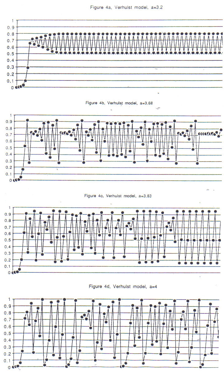
Figure 4a-d: Verhulst Model

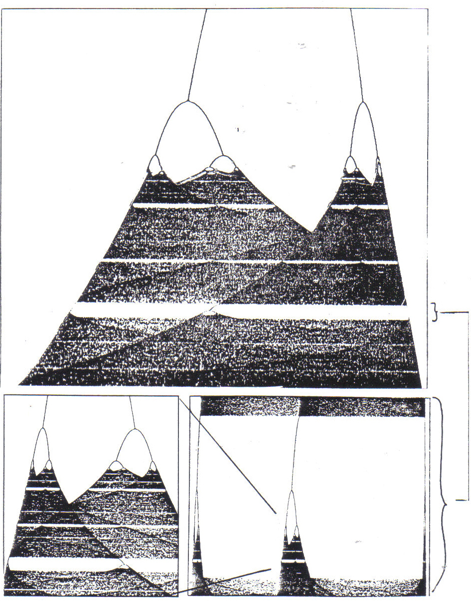
Figure 4e: Verhulst Model: all "a" values along x axis.

To compose Fractal Piano 6, values obtained from iteration of the Verhulst formula where encoded into MIDI-data in the form of pitches, lengths and loudnesses. The mapping of x values to a given parameter was not direct, proportional, or linear: rather, musically more interesting results were obtained with a "scrambled" mapping (like a partially "shuffled" scale), or with a selected or weighted element set. "Note" data was combined and "scored" with the help of a commercial sequencer program: then stretched or squeezed time-wise and layered and edited in various ways using "fractal" structures. For example, the on/off pattern shown in Figure 5 was used as a mask to create a kind of crescendo in one part of the piece. The upper register of the piano turns on and off at intervals of 2 seconds. When this register in "on", material is audible within this register; when it is "off", it is silent. In a register just under the highest one, the mask turns on and off every 4 seconds: in a register just under it, every 8 seconds, and so on. By applying such a mask over the (potentially endless) chaotic material, I find a kind of musical tension is generated. Notice that the whole mask pattern produces all possible combinations of "on" and "off" for the chosen number of registers. It is related to the I Ching, with its 64 possible combinations of 6 solid or broken lines. (Sound example 3.)

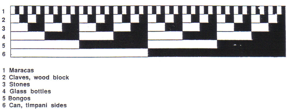
Figure 5: Combined Scheme for Fractal PIano 6 and "The Five Seasons", Aftersummer.

"Fractal" is a term coined by the Polish-born mathematician Benoit Mandelbrot. He derived it from the Latin adjective fractus, meaning irregular or broken. Fractals are characterized by intricately nested patterns within patterns with self similarity on any scale. Fractals can be recognized in a wide range of natural phenomena and shapes, such as trees and clouds. Analysis of Indonesian gamelan music reveals tree-like patterns which are essentially fractal. (See Figure 6.) The rhythmic punctuations fits a pattern based on the series 2,4,6,8,16 etc. and the nuclear melody is performed on several different instruments at different speeds.

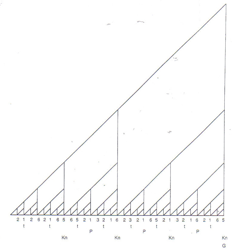
Figure 6: Javanese Gamelan: t = Ketuk, P = Kempui, Kn = Kenong, G= Gong, 2 1 2 etc. = Balungan (nuclear melody) played on Saron/Sientem

Fractals can also be generated using simple rules to make geometrical monsters, such as Cantor Dust and the Koch Snowflake. (Figures 7a-b.)

Figure 7a: Cantor Dust (from Benoit Mandlebrot, Fractal Geometry of Nature, reproduced with permission.

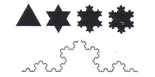
Figure 7b: Koch Snowflake (from Chaos, by Thomas Bleick, reproduced

Mandelbrot's great contribution was the realization that whether one was considering bursts of noise on telephone transmission lines, stock market prices, or Cantor Dust, the degree of roughness or irregularity could be defined mathematically by a "fractional dimension." To get a feeling for this fractional dimension, think of the construction of the Koch Snowflake (fig.7b); it starts out as a one-dimensional line, but as we go on adding infinitely many ever-smaller triangles, the jaggedness begins to fill up a two-dimensional surface. Mandelbrot calculates its dimension to be 1.26... . Likewise, intuitively we can appreciate the calculated dimension of Cantor Dust (Figure 7a), which is 0.63; considered as a whole, the collection is somewhere between the dimension of a point, namely zero, and the dimension of a line, namely 1.

Although the degree of irregularity of an outline could now be calculated and found to be constant regardless of whether we sample a small or big piece of it, we discover that the question "How long is it?" becomes meaningless. In answer to the question, "How long is the coastline of Britain?", Mandelbrot answers that it depends on the length of your measuring stick. As you decrease the length of your stick, you measure more nooks and crannies of the coastline, so your total measurement appears to become longer. If your unit length is infinitely small, the coastline becomes infinitely long!

Since the publication of Mandelbrot's "The Fractal Geometry of Nature" his name has become attached to a certain analysis called the "Julia Set". The French mathematician Gaston Julia wrote a paper in 1919 about a set of iterative equations:

X_n+1 = x²_n - y²_n + a

Y_n+1 = 2x_ny_n + b

The equation-pair produces transformation of a planar point, labeled (x_{n, yn}) into a new point (x_n+1, y_n+1). For any arbitrarily chosen values, of a and b, we get a fractal when we investigate what the equations do. Starting from any point (x₀, y₀) we calculate new points repeatedly, plugging results back into the equations, and observe one of two things: either the values tend to jump around in (sometimes chaotic) orbits; or they fly off toward infinity. Using a computer one can then make a picture of what happens to all starting points in the x-y plane, coloring an initial point if it results in a stream of finite numbers, for example.

All Julia fractals show point-symmetry with regard to the origin (0,0). One is reminded of the swirls and curlicues of rococo architectural decoration. When b=0, they have mirror-symmetry as well; one member of the set has been fancifully called "San Marco" because it resembles the famous Basilica in Venice, together with its reflection in a flooded Piazza. Depending on what one chooses for a and b, the resulting graphic falls into one of two classes: connected or dis-connected. The disconnected sets are planar analogues of Cantor Dust (previously described): clumps or clusters of points.

Mandelbrots's Set is a kind of catalog of all Julia Sets, showing which values of a and b produce either a connected or disconnected Julia Set. To simplify calculation, "imaginary numbers" are used. A plot is made on the a-b plane. Initially, we set x₀=a and y₀=b. After say, 100 iterations of Julia's equations, it is determined whether the x and y values are heading toward infinity, and if so, how fast: the initial point (x₀, y₀) is then given a color coding of some kind. If the values don't head toward infinity, the initial point remains black. The colored points correspond to Julia sets of the disconnected type and points within the black cardiode figure correspond to Julia sets of the connected type.

Mandelbrot's set is claimed to be one of the most complicated structures known to mathematics. Computer graphics show it to contain an infinity of twisted, swirling, grotesque baroque forms; it is frighteningly beautiful. One can use the computer like a microscope; zooming in to a seemingly isolated point "outside" the central black area, one discovers the shape of the original whole Mandelbrot set. Mandelbrot's set is therefore a fractal, too. However not without certain mysteries as it was recently proved that all the island universes are actually connected with the main body with thin filaments. (See Figure 8a-b.)

I have come to think of the improvisor and instrument combination as a kind of feedback system. The "output" of instruments enters the performers' brains where those mysterious processes occur which allow them to produce new output. We have seen that mathematical feedback loops are at the core of the Verhulst Model, the Julia and Mandelbrot Sets. There are indications that almost any complex organization; whether it is of cells, body organs, individuals, or the groups of groups we call corporations nations, etc.; all require some kind of feedback for healthy stability.

Flocking animals coordinate in a remarkable and still incompletely understood fashion. The reaction time of a group in danger, or in making turns is considerably faster than the reaction time measured of isolated individuals. Still, it is evident that in order to maintain the proper distances between neighbors without collision, some sort of multi-sensory positive-negative feedback mechanism is in operation. LIkewise, neural physiology has revealed that the massively interconnected neural network in the brain also operates with feedback processes. A neuron cell has a main body; an axon from which it receives signals; and tree-like extensions called dendrites which branch off in hundreds to make contact with other cells. Connections between axons and dendrites are effected across gaps, called synapses. Neurons send out impulses spontaneously at a rate of about 10 a second. However, the rate of firing changes, and depends on the sum total number and strength of the impulses it receives. There are both excitatory and inhibitory synapses; signals from the former tend to increase the firing rate of a cell, while the latter tend to reduce the firing rate of a cell. The picture of ceaseless electrical activity - signals amplifying, muting modulating, crossing each other and returning in loops; all incredibly complex and indecipherable wave-like patterns - this picture gives us an idea of how thought and memory are possible. Recent investigation of the physiology of perception has led to the discovery of chaos in the brain; complex behavior which seems random, but has a hidden order. Vast collections of neurons shift quickly from one complex pattern to another, in response to the smallest of inputs (remember the butterfly effect). An organism as a whole acts in its environment with feedback mechanisms. The brain seeks information and spreads signals to muscles to place sensory organs in position and to sensitize parts of the brain which swill process signals.

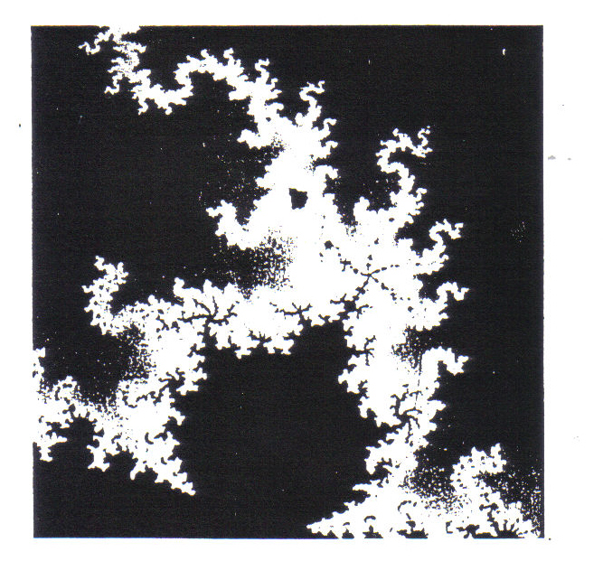
Figure 8a: Mandlebrot Set

A burst of collective patterned activity from all sensory organs is combined to form a gestalt. Then a fraction of a second later, another search for information is demanded. It seems that chaos in the brain is not pathological, as one might expect, but instead is the basis of healthy functioning; this indeed explains how the brain can respond quickly and flexibly to an ever-changing outside world. Even what we experience as a original idea (brain-storm) may be derived from a chaotic neural firing pattern triggered in an ever-widening cascade from a small initial impulse.

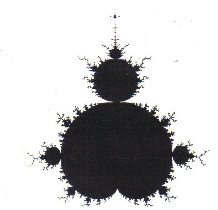
Figure 8b: Mandlebrot Set (detail) from Fractals by Hans Lauweries, reproduced with permission)

In my piece Brain Wave for at least 3 recorders of any kind, (1989), I wanted to set up a self-regulating musical situation. All musicians improvise on the same basic material, which is arranged in four cycles, each with four events. (See Figure 9.) Performers should stand or sit spread out around the hall, possibly on different levels. Each player should face an arbitrarily chosen direction. Emphasis is placed on influences which performers take from their neighbors. Players in front of an individual project positive influences, and player(s) in back give negative influences. A crude summary of how these influences may be conceived is summarized in the following table:

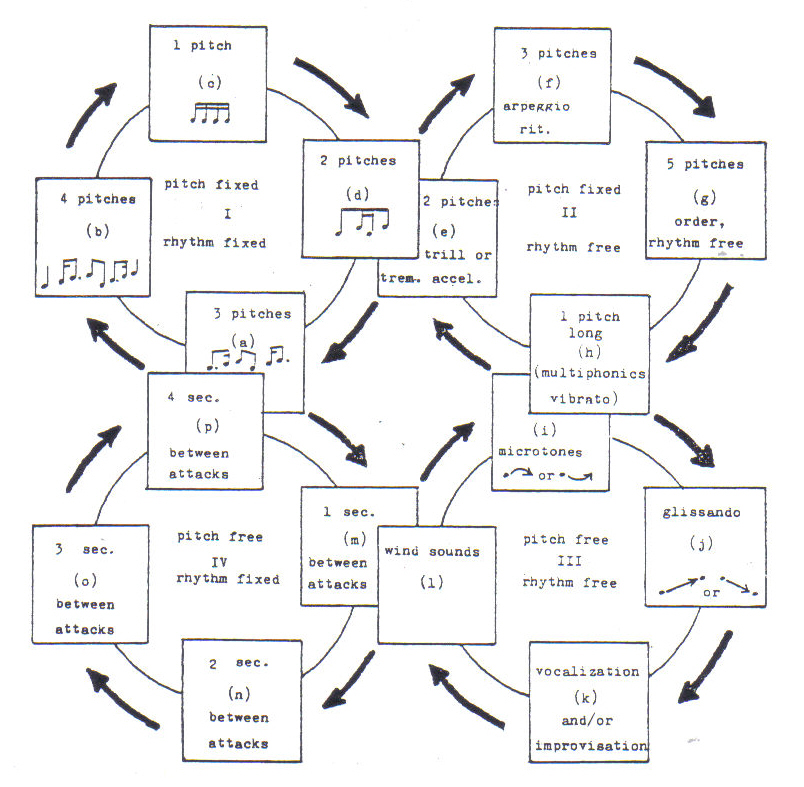
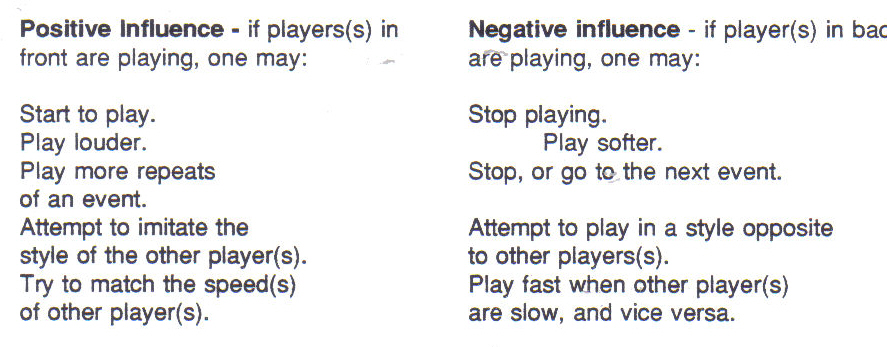
Figure 9: Brain Wave

The object is not to synchronize exactly with the other players, but to correlate what a player does with what the others do. Since there is no conductor, each player must partly assume that function, being attentive to the ensemble sound, and taking initiative to lead that sound where he/she thinks it should go. The aim was to create an interactive situation such as is found in nature, among flocks of birds, or in brain neurons, for example. (Sound example D.)

In 1989 I completed The Five Seasons for 6 percussionists and tape. My inspiration source was an ancient Chinese theory, in which the Seasons, Emotions, Colors, Elements and Directions were grouped as follows (Figure 10.)

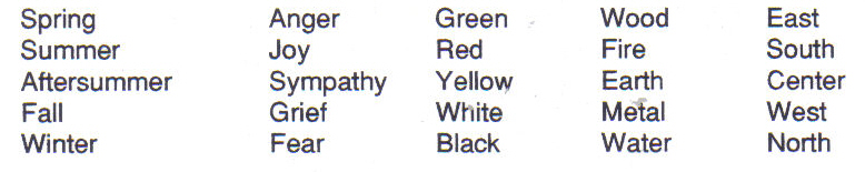
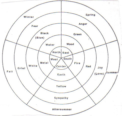
Figure 10: The Five Seasons Classification Scheme

This piece incorporates several techniques which were derived from Chaos Science. My adaptation of the Verhulst Model was used to derive some of the rhythmic materials for the piece as in Fractal Piano 6. Fractal structures define the form of several sections. Some of the electronic sounds on the tape were made using feedback loops for frequency modulation. The performers are called on to improvise in one section.

The first part Spring, begins with accelerandos of accelerandos. First a pulse plan was worked out; the distance between pulses starts large, with successive pulses scaled by a ratio such as 2/3rds down to small (fast) intervals. Then an accelerating figure was fitted to each of the pulses.

(A similar slowly accelerating roll is found in Chinese opera and Korean ceremonial music.) There are three layers, played by wood blocks, temple blocks, and log drum. Later on, a 16 note theme in quarter notes is introduced in the bass marimba. The melodic curve of this theme is a projection of a fractal graphic design I made. Here a 4-note melodic motive is fitted or transposed into a blown-up version of itself. (See Figure 11.)

Figure 11: The Five Seasons (theme).

Such nested patterns with scaled elements are characteristic of fractals, as already described. There follows a metric canon; the theme enters in eighth notes, then triplet eighths, and finally sixteenths. One can consider the whole construction of metric canons as a fractal of a fractal, since the theme pattern (itself a fractal) occurs simultaneously at different speeds and octaves. After another metric canon and a section with controlled improvisation, this theme returns with a different treatment. It is split up into 4-note fragments and given a peculiar "doubling" not parallelism, but an exaggeration of the melodic curve, using multiplication. Again, such "scaling" is a common method of constructing geometrical fractals. (See Figure 12. Play example E.)

Figure 13 is a wiring scheme used in electronic FM synthesis, in the second part, Summer. This scheme includes two feedback loops: the output of any generator provides input control voltages for two other generators. A positive arrow indicates that when the voltage output of a Low-Frequency Oscillator (LFO) is high, it causes its neighbor LFO to oscillate at a higher rate. The negative arrows indicate that inverted signals are sent out. In this case a high output voltage of a LFO causes a lower rate of oscillation in a cross-connected LFO. One may also use the output of any or all of the LFO's for control of other electronic devices, to synthesize a sound. Because of the interconnectedness, and the complex interaction of positive and negative feedback loops, the results of such a circuit can be unpredictable and chaotic. The second part, Summer, is itself divided into four sections, each with a clearly defined instrumentation. Each section and all instruments have similar material, rhythmically, generated from my computer program using the Verhulst Model. (Sound example F.)

The third part, Aftersummer, uses the on/off masking scheme used also in Fractal Piano 6. Here, not registers on the piano, but six different percussion timbres (all with a sharp decay) are "turned on or off". As in Fractal PIano 6, we get all 64 possible combinations of the six elements, and a kind of crescendo. (See Figure 5 again, and sound example G.)

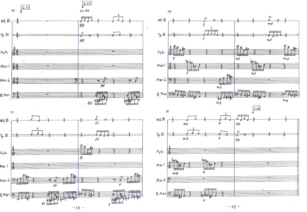
Figure 12: The Five Seasons p.14,15.

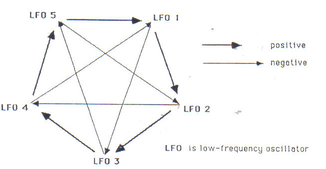
Figure 13: Feedback Loops for Electronic Synthesis.

The fourth part, Fall, depicts musically the "Butterfly Effect", previously described. In the last measures of Aftersummer, all six players have finally come together. In the first measure of Fall, they play all together again (this time on metal instruments); and then disperse. Sometimes 2 or 3 players synchronize for a while, but small deviations lead to larger separations, and this part ends fragmented and scattered. Loosely spoken, this part is an inversion of how Spring begins. Fall contains a ritardando of ritardandos. (Sound example H.)

For the fifth and last part, Winter, I used a technique I call "nested repeats" to create the metric structure; it proves to be a fractal. Difficult for a human perhaps, but a computer can easily carry out the set of commands shown in Figure 14.

j+[h+[f+[d+[b+[a]+c]+e]+g]+l]+k =

jhfdbaacbaacedbaacbaacegfdbaacbaacedbaacbaaceglhfdbaacbaacedbaacbaacefdbaacbgaacbaacegik

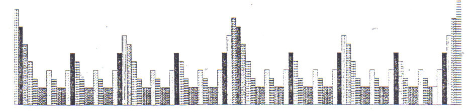
Figure 14: Nested Repeats

Here the [] signs indicate a simple repetition. [a]= aa for example. The nesting of the repeats makes that a get printed 32 times, b and c 16 times, d and e 8 times, f and g 4 times, h and i 2 times; and j and k get printed only once each. Whether you look at a small or large part of the list above, it displays the self-similarity typical of a fractal.

For Winter, I desired a metrical structure with many changes but internally consistent. First I decided what was going to happen in each measure, in terms of instrumentation and so on, and then let the length in eight-notes per measure be determined by substituting the numbers 2-12 for a-k in the fractal pattern. (See Figure 14, sound example l.)

The last piece I'd like to discuss here is Modi-fications for large marimba and tape, (1990). WIth this piece, I made use of what I call "transposing modes". These are constructed like fractals with an interval structure repeated indefinitely. For example, take the interval cell [1,4,2] (semitone = 1). Starting with a low E and repeating the cell, we get E F A B C E F#. Notice that because the elements of the cell add up to 7, two cells don't complete an octave, but overreach it. Indeed, we must repeat the cell 12 times before we get the same pitch-names. Playing "scales" up or down through this mode, we get continuous transposition through the cycle of fifths.

The ordering of much of the materials in the piece was achieved with a computer program which I worked out called "statistical feedback". Here use is made of weighted random choice between elements; only the order of preference among elements is always changing, depending on previous choices. For example, suppose we have 4 elements abcd. We enter them in that order into the computer memory. The computer then makes a weighted random choice among them; it has an increasing preference toward the last items on the list, and would avoid choosing the first item a. Suppose it chooses d. Then d is placed at the beginning of the list. The memory then contains dabc. Again the computer chooses with increasing preference toward the end of the list; this time we get a. The ordering changes again: adbc. Figure 15 shows the results of several cycles of this program, together with the computer's memory state.

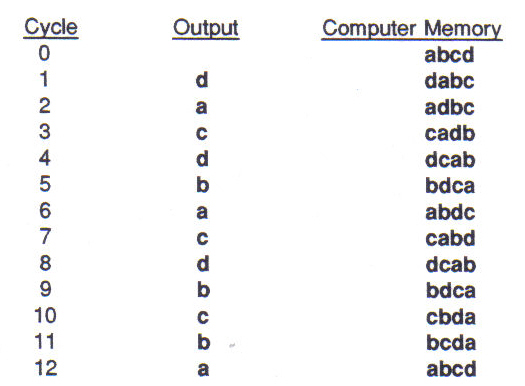
Figure 15: Statistical Feedback

Even though we have arrived at the initial memory state after 12 cycles, it is unlikely that we will get the same sequence if we continue to run the program. What it does is make a "chaotisation" of serialism. I have used this program on several different element sets in composing the marimba part as well as the tape part of this piece. Pitch, note length, dynamic, as well as larger structures: mode, section length, and electronic timbre; all material and forms are subject to Modi-fications. (Sound example J.)

In closing this presentation, I must emphasize that my aim in using techniques derived from chaos sciences has not been to make totally automated music. A composer must make choices on many levels; any technique properly used remains only a tool in the realization of his/her ideas, fantasies and feelings. Still, the new discoveries and techniques open up new worlds beyond even our imagination. I believe in particular, that composers may do well to take a new look at chaos.

References

Capra, Fritjof: The Tao of Physics; 1976 Bantam Books.

Dewdney, A.K.; "Wallpaper for the Mind: Computer Recreations," Scientific American,September 1986.

Freeman, Walter J.: "The Physiology of Perception," Scientific American February 1991.

Gleich, James: Chaos, Making a New Science, Viking Press 1987.

Hawking, Stephen W.: A Brief History of Time, Bantam Books, 1988.

Hofstater, Douglas R.,: Gцdel, Escher, Bach; Vintage Books 1980.

_________________; "Metamagical Themas," Scientific American November 1981. (from Mathematical Chaos and Strange Attractors, Penguin Books, 1987.)

Lauwerier, Hans: Fractals; Aramith, 1987.

Mandlebrot, Benoit: The Fractal Geometry of Nature; W.H. Freeman and Co. 1983.

Prigogine, Ilya: Order out of Chaos; Fontana Paperbacks, 1985.

Russel, Peter: The Brain Book; 1979 Routledge.

Watson, Lyall: The Dreams of Dragons; 1987 Morrow, New York.