Music From Chaos:
Nonlinear Dynamic Systems as Generators of
Rick Bidlack
In recent decades, a great deal of
attention from the scientific and mathematical
communities
has been focused on the exploration of a class of mathematical objects known
as
nonlinear dynamical systems. Although the symbolic specification of many of
these systems
is simple to the point of apparent triviality, their behavior can often be
extremely rich
and complex, even unpredictable.
This
unpredictability, arising as it
does from processes
which are completely deterministic, has a certain flavor to it which is
quite distinct from the uncorrelated
randomness of white noise or other probabilistic distributions. The generic
term for this brand of deterministic
unpredictability is chaos,
and the body of
theory which describes
it is often called chaos theory.
(The terms 'nonlinear dynamical system,' `chaotic
dynamical system,' or simply 'chaotic system,' are considered in the present
context to be synonymous.) Nonlinear dynamical systems are interesting to
scientists because they exhibit structural
characteristics which are shared by forms found in nature. Chaotic systems are thought to underlie or model important aspects of
the motion (change in location) and/or evolution (change in form) over time of
phenomena in the real world. The complexity of behavior exhibited by certain chaotic mathematical objects - specified
as sets of equations -rivals that of real-world phenomena in many
instances.
The meshing of a number of events has raised the subject of chaos to its
currently
topical level within the scientific community. Improved methods for the
analysis and theoretical description of
dynamical systems were developed around the turn of the century by Poincaré and others. The advent of cheap
and plentiful computers has made practical the computation and analysis of numerical solutions to nonlinear
equations. Moreover, computers have made graphical representations of
the behaviors of these systems possible, revealing extraordinary structures
which would not immediately be apparent from the raw numerical data. Today,
increasingly well-defined behavioral and structural parallels between chaotic
systems and real-world phenomena are being found and described. The range of phenomena which are presently being studied in
terms of underlying chaotic structure is diverse, and includes: fluid
flow, aerodynamics and turbulence2, orbital deviations and
The
exploration of chaos is forcing a change in the definition of this word. Chaos is
not
formless anarchism, it is a highly structured phenomenon
pervasive throughout the natural world. Its variations are
rich and complex, and
its properties are intriguing. Its
study has invigorated
large segments of the mathematical and scientific communities; perhaps it has
the potential to inspire artistic activities
as well.
Nonlinearity is a concept which is intuitively understood and
applied in a wide range of everyday
situations. The popular adage about the straw that breaks the camel's back is based on this understanding. In this
quintessentially nonlinear situation, a small quantitative
change to the "input" (the addition of
one straw) is seen to cause a dramatic qualitative change
in the "output" (the demise of the camel). Another example, used by
Glieck13, is the traditional verse:
For want of a nail the shoe was lost.
For want of a shoe the horse was lost.
For want of a horse the rider was lost.
For want of a rider the battle was
lost.
For want of a battle the kingdom was lost.
This is a
perfect example of what is more formally known as sensitive dependence on initial conditions,
the idea that
a seemingly insignificant variance at the outset of a chain of events may
nonetheless precipitate effects down the line that build up to irrevocably and
drastically
alter
the final outcome. One might also think of the performance of the economy (seemingly
immune to all theory and attempts at regulation), the occurrence of earthquakes
(sudden jolts resulting from presumably
constant tectonic pressures), or even the outbreak of war (an abrupt shift of international tension from the
political to the military arena) as familiar examples of nonlinear
dynamics at work.
Nonlinear dynamical systems are mathematical objects which behave in
similarly unpredictable ways. To understand how these expressions
can be manipulated to produce musical
results, certain basic concepts of dynamics and nonlinear equations must
be understood. Among the terms to be introduced in this section and in
the following chapters are: phase space,
orbit, bifurcation, attraction,
dissipative and conservative systems, transients,
sensitive dependence on initial conditions, Poincaró section, iterated
map and continuous flow. An operational
definition of chaos, if not a rigorously mathematical one, will
hopefully follow from a familiarity with these concepts.
Dynamical systems convey in their
notation an implicit recognition of the passage of time. The length of time that passes is
rather arbitrary; what is more important is the quality of the time, or how it is
fundamentally conceived. If the mathematical expression of a dynamical system implies the
passage of time in terms of discrete steps of a uniform
size, then the system is a difference
equation,
of the form
xt+1 = f(xt)
This
is akin to a simple feedback system, in which the current output of the equation
becomes the
input for the next iteration. Systems expressed as difference equations are
also called iterated
maps,
because the effect of the equation is to map one value, xt,
to another value,
xt+1, for each iteration of the equation. If, on the
other hand, time is considered to be a continuous quantity, advancing smoothly, then
the system is expressed as a differential
equation
in the form
x = dx1dt = f(x),
where x
is a measure of the rate of
change of the dependent variable x with respect to time.
These
systems are called continuous flows,
and
what they produce are smooth, unbroken
curves. In a digital computer,
however, continuous time cannot exist - it is a theoretical concept that must be approximated in simulation.
This is accomplished by reformulating the differential equations of the system into difference equations, a
process called integration. Several
methods have been developed for integrating differential equations, but only
the simplest of these, Euler's
method, is used in this study. Essentially, this procedure calculates a value (x)„ from the function f(xn),
then
computes a new x
based on this value according
to the
formula
xn+1 =
xn +
xn
∆t,
where Delta t is typically a very small value, 0.01 or less. The effect
of this procedure is to
move forward along the curve by very
small, discrete steps (of unequal length, but equally
spaced in time.)
In mathematical terms, nonlinear equations are simply those which are
not linear.
Linear algebraic
equations
are those in which the degree of the variables is unity, e.g., none of the
variables of the equation are raised to any power other than one. An example is
the linear equation y = mx b,
which defines a straight line of slope m
and y-intercept b.
On the other hand,the
second-degree equation 9 = mx b,
which defines a parabola,
is not linear. This distinction applies in differential
equations
as well, although in
this case the only variables for which
the degree is significant are the dependent
variables,
the ones for
which a derivative term occurs in the equation. For example, the equation
x2 (dy/dx)
+ y(x3 - 2) = 2x3
is linear in y,
even
though x
is both squared and cubed, because the
dependent variable y
is always of degree one. The
equation
A(dy2,/dx2) + B(dy/x) + Cy3 = cos(x)
is nonlinear in y
because the
dependent variable y
is raised to the
third power.
While the degree of an equation is critical in the distinction between linear and nonlinear dynamical systems, it is not the only factor in determining whether or not a given equation is nonlinear. The presence within an equation of a trigonometric function, or, in a differential equation, the multiplication of two or more of the dependent variables with one another, are also sufficient causes to make the equation nonlinear.
One of the simplest nonlinear equations known to exhibit chaotic behavior is the logistic difference equation, also known as the quadratic or parabolic equation. This equation has been applied in studies of the population dynamics of a species from generation to generation14. It specifies the population P at successive time increments 0, 1, 2, ... ,n as a function of its prior value:
Pn+1 = KPn(1 - Pn),
where K is a parameter whose value normally remains constant once an iteration sequence is initiated. The equation is nonlinear by virtue of the quantity P2 (remember that K P (1 - P) = K P - K P2). Despite its apparent simplicity, the dynamics of this equation are sufficiently complex to have warranted attention from many authors in the mathematical community; see for example Thompson and Stewart15, Ruelle16, Devaney17 and Moon18.
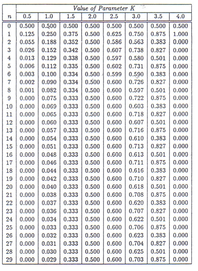
The equation may be iterated indefinitely, to produce an arbitrarily long sequence of numbers Po, •" Rn• This sequence is called the orbit or trajectory. The term orbit does not necessarily imply a smooth, continuous curve. While the orbit of the earth around the sun may be quite smooth, orbits of iterated maps such as the logistic function can be quite erratic. The equation becomes interesting when the orbits resulting from the adoption of different values for the constant K are compared. Table 1 lists the first thirty iterates of eight different orbits, each following from a different value for K. Although the initial value P0 .5 in all cases, each orbit is quite distinct from the others.
Three distinctly different modes of behavior are demonstrated by the orbits shown in Table 1. First, for K-values of 0.5, 1.0, 1.5, 2.0,2.5 and 4.0, the orbit is drawn to a single point, or fixed point, where it remains. (For K =1.0, the orbit is eventually drawn to 0.) This point is called an attractor. The rate at which the sequence of values converges on the single-point attractor varies from immediate (K 2.0) to extremely gradual (K = 1.0). Secondly, for K. 3.5, the orbit is attracted to a limit cycle, where it oscillates indefinitely. In this case, the limit cycle is a periodic oscillation among four points. This is a periodic attractor. Third, for K. 3.0, the orbit describes a damped oscillation wherein the high and low values converge asymptotically. The two values will converge to a single point only when the limit of resolution of the program which is computing the orbit is reached - in other words, when the computer is no longer able to make a distinction between the two values. Depending on what this resolution is, this may not occur until after tens of thousands of iterations have been calculated.
Table 2 shows the first eighty iterations of eight more orbits of the logistic equation, each from an initial point P0 = .5, for values of K starting at 3.55 and increasing in steps of 0.01125. These orbits illustrate modes of behavior which are again quite distinct from those shown in Table 1. Within the span of eighty iterations listed, only two of the orbits attain an unambiguously periodic state: the first, for K 3.55, and the last, for K 3.62875. In both of these cases, the P-values comprising each cycle do not repeat exactly until after the sixtieth iteration. The initial portion of the orbit, during which the eventual, settled behavior of the equation under the specified conditions (the value of the parameter K and the initial value of P) is approached, is called the transient segment of the orbit. In the case of these two periodic orbits, the span of latent periodicity prior to the sixtieth iteration (approximately) comprises the transient portion. For the orbits shown in Table 1 which are attracted to a single point, the transient state consists of those points through which the orbit passes before it settles onto the fixed point. There is not necessarily a firm dividing line between the transient portion of an orbit and its settled state. Some orbits ease into their settled behaviors very gradually, while others show no transients at all.
Four other orbits in Table 2 appear to be headed toward a regime of periodicity, but none of them reaches this state within the span of eighty iterations shown here. For K = 3.56125, the orbit tends toward a period 8 oscillation. For K = 3.57250 the tendency is toward a period 24 oscillation, for K = 3.58375 it could be a period 12 (although it gets "noisier" rather than cleaner as it progresses), and for K 3.60625 there is a clear period 10 oscillation. In practice, it is sometimes difficult to determine whether or not a given orbit is being attracted to a periodic state without following the orbit for a much longer span than has been illustrated in Table 2. These orbits may still be in a transient state, headed toward an ultimately periodic condition; on the other hand, it is possible that one or more of them has already settled into a long-term state of "noisy periodicity" within the span shown here. Adding to the ambiguity is the fact that a determination of a given orbit's periodicity is contingent on the numerical resolution used in the representation of that orbit. Long transient orbits appear to become shorter when fewer significant figures after the decimal point are used. On the other hand, the seemingly exact periodicities finally attained in the first and eighth orbits may simply be artifacts of there being only five significant figures after the decimal point.
Table 1:
Eight orbits of the logistic equation, in numerical form for different values
of
the parameter
K.
All orbits begin
at the same point P0 = 0.5.
The remaining two orbits in Table 2, for K = 3.595 and K = 3.61750, tend neither toward a fixed point, nor to a limit cycle. These are chaotic orbits, in which the sequence of values is quite erratic, and apparently random. The fact that these orbits are the result of a completely deterministic procedure (the equation itself) is one distinction between true randomness and chaos.
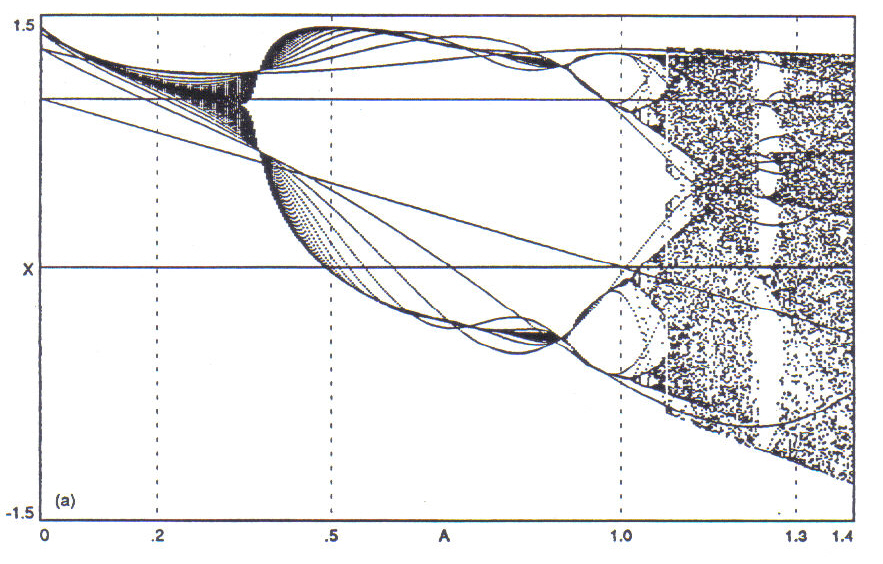
Taken together, Tables 1 and 2 demonstrate a remarkably rich (and potentially bewildering) range of behavior for an equation as apparently trivial as the logistic equation. Graphical methods of representation may be employed to clarify this behavior and relate it within a global context. One method is the construction of a bifurcation diagram, in which a large number of partial orbits are computed and plotted against a range of values of the constant parameter. Figure 1 shows two versions of a bifurcation diagram for the logistic equation over the range 0 < K < 4. In the first version, the first 150 points of each orbit are plotted, while in the second version iterations 150 through 300 are plotted. Thus, the first version illustrates the transient behavior of the system, while the second version shows the settled behavior (this assumes that most transients have died down by the 150th iteration). Figure 2 shows two successive magnifications of the diagram, the first in the range 3 < K < 4, the second in the range 3.55 < K < 3.62875. Several important features of the behavior of the logistic equation emerge from an examination of these diagrams. When the value of K is less than 3.0, the orbit is attracted to a single point (for K < 1, this point is 0). At K = 3.0, a bifurcation of the attractor is evident. At K apx. 3.46, a further bifurcation is seen, forming a period 4 oscillation (compare Table 1, for the orbit at K = 3.5). Yet another bifurcation occurs just before K= 3.55, and again between 3.56125 and 3.5725. The period of the oscillation is thus doubled at each bifurcation node, in a sequence called the period-doubling cascade. Eventually, the nature of the attractor undergoes a change from a condition of periodicity to one of chaos. For the logistic equation, the chaotic regime begins at around K 3.567 and extends to the maximum value of K 4.0 (orbits at higher values of K are unstable). Nonetheless, periodic windows are found interspersed throughout the chaotic regime; note, for example, the large period 3 window around K 3.84. Figure 2(b) provides a new perspective on the eight orbits listed in Table 2. The period 24 window at K = 3.5725 is barely discernible, while the period 12 orbit at K 3.58375 is seen to lie right on the edge of a periodic window. Chaotic orbits for K 3.595 and K 3.6175 lie squarely within chaotic regimes.
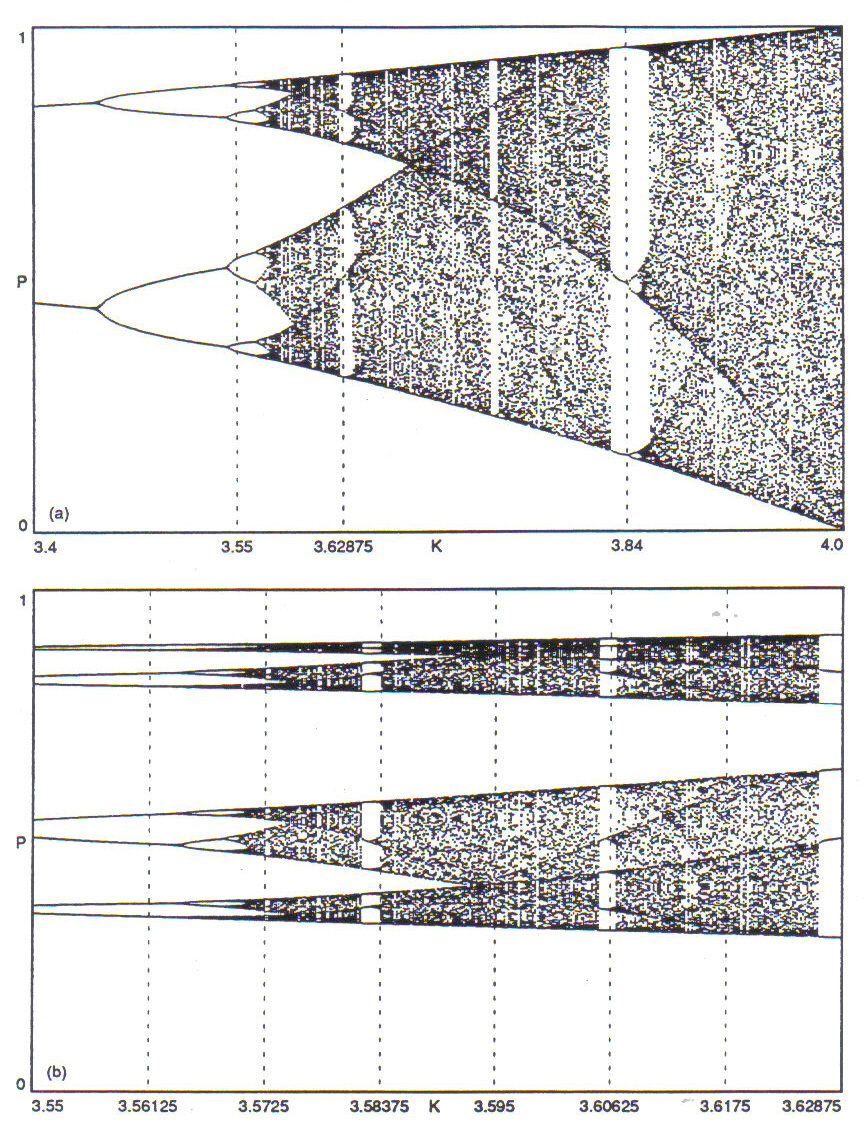
Figure 1: Bifurcation diagrams of the
logistic equation, over the range 0 <
K <
4, with
PO
.5;
(a) showing transient behavior (first 150 iterations),
(b) showing settled behavior (next 150 iterations).
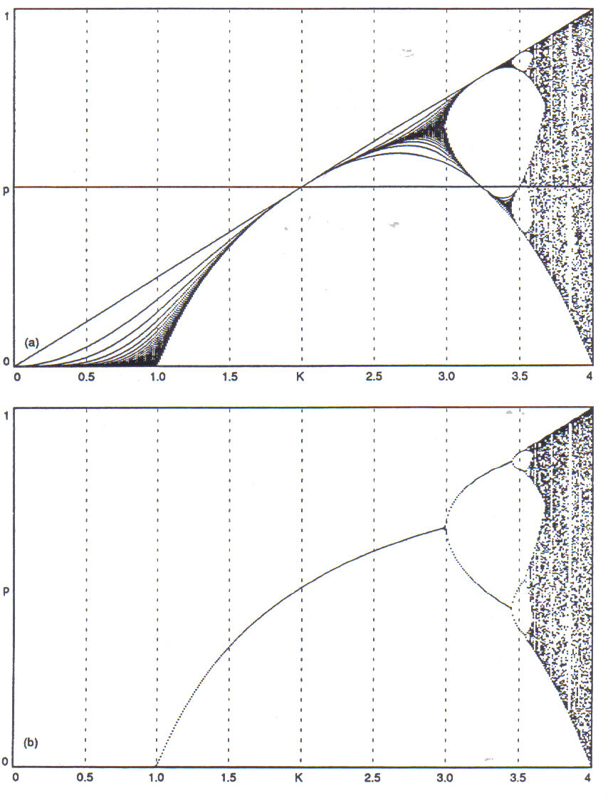
Figure 2: Magnification sequence of bifurcation diagrams of the logistic equation; (a) in the range 3 < K < 4, (b) in the range 3.55 < K < 3.62875. Iterations 150 through 300 are plotted.
Thus far, all of the numerical orbits listed, as well as the four bifurcation diagrams plotted, have been initiated from P0 = 0.5. In fact, any initial value of Po between 0 and 1 could have been used to produce basically the same results. For those values of K which lead to periodic orbits, only the initial transient portions of the orbits would be different. For those values of K which lead to chaotic orbits, the exact sequence of points along the orbit would be quite different for different values of Po, but the range of values over which the orbit wanders would remain the same. Thus, the two bifurcation diagrams in Figure 2, which do not plot the transient portion of the orbits, would look essentially the same no matter what the initial value of Po. This is the significance of the term attractor - orbits are drawn to the same attractor regardless of their respective starting positions as long as the parameter values (just K in this case) are equivalent. (There are exceptions to this rule. In certain situations, different initial conditions may lead to different attractors under the same parameter values. An example of this follows, and another is included in the discussion of the Hénon map in the next chapter.)
Another intriguing aspect of chaotic orbits is their sensitive dependence on initial conditions. Two orbits which begin at almost the same point will eventually diverge from one another. An example of this is shown in Table 3. Here two orbits are followed through twenty-four iterations. For both orbits, K 4.0, while the initial value Po differs by only 1/100,000. Nonetheless, this difference causes a complete divergence of the two orbits within the span of fourteen iterations. This effect can be demonstrated with any chaotic dynamical system, no matter how small the initial difference. Incidentally, a comparison of these two orbits with the last orbit listed in Table 1 (for K 4.0) demonstrates the effect mentioned above, that co-existing attractors may emerge for different initial conditions.
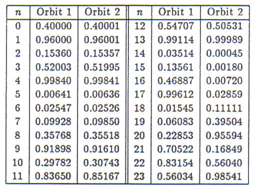
Table 3: Two orbits of the logistic equation, demonstrating sensitive dependence on initial conditions. K. 4.0 for both orbits, while P0 differs only by 1/100,000. The orbits remain fairly similar through fourteen iterations.
The phenomenon of sensitive dependence on initial conditions has wide-ranging ramifications for anyone working with chaotic systems. Since real numbers can only be represented with finite precision in a computer, rounding errors in the calculation of any orbit are inevitable. These errors eventually accumulate, causing the calculated orbit to diverge exponentially from the theoretical orbit. Slight differences in the implementation of an algorithm to compute an orbit (for example, the order in which mathematical operations are carried out), the precision employed, or the use of a different computer, are sufficient to cause a divergence of trajectories. One may rely on the global behavior of a chaotic system to remain roughly the same from machine to machine, but not the precise sequence of a given orbit.
This study approaches the issue of the generation of musical materials by means of nonlinear dynamical systems through an examination of two distinct systems: the Hénon map and the Lorenz system. These systems, only slightly more complex than the logistic equation just discussed, were chosen not only because they are well-known and widely studied, but because they are exemplary of certain fundamental classifications of nonlinear dynamical systems in general.
The Hénon map is an iterated map, an object in which the passage of time is represented in discrete steps of equal size, as would be appropriate in the periodic measurements of things such as populations, water levels, or stock prices. The phase space, or the area in which the dynamics of the system take place, is two-dimensional. In the case of the Hénon map, the significant portion of the phase space may be represented on the Cartesian plane, between approximately -1 .5 and 1 .5 on the x-axis, and between approximately -0.4 and 0.4 on the y-axis.
The Lorenz system is a continuous flow, a phenomenon in which the passage of time is - theoretically - represented in an unbroken manner, as would be appropriate to the calculation of celestial orbits or to the representation of wind speeds over a continuous span of time. The stable phase space of the Lorenz attractor is three-dimensional, roughly symmetrical around the origin along both x and y axes, and lying entirely in the positive region along the z-axis.
The Hénon and Lorenz systems are dissipative, that is, they are representatives of a class of phenomena in which the total energy of the system is dissipated over time. (The logistic equation is also a member of this class.) In analytic terms, this means that the phase space of the system shrinks over time. The dissipation of energy occurs during the initial transient portion of the orbit. Orbits of dissipative systems are drawn to an attractor, which may be either a point (a single-point attractor), a set of points (a limit cycle or periodic attractor), or a complexly folded region of space (a chaotic attractor or strange attractor). The great majority of earth-bound dynamical systems are dissipative, due to energy loss through friction.
Other systems not discussed here are conservative. They are representative of phenomena in which friction does not play a role, those in which energy is conserved. These systems are also called Hamiltonian systems or area preserving systems, because their phase spaces do not shrink with time. Thus, they cannot properly be said to have an attractor, although they do exhibit periodic and chaotic behaviors in a manner parallel to that of the dissipative systems. Such systems occur within the realm of celestial mechanics, and on earth, within the electromagnetic storage rings of particle accelerators.
The Experimental Apparatus
It is desirable, in an initial exploration of a potential compositional technique,that highly subjective issues be removed from the picture, or at least minimized as much as possible. The question at hand is not: "How can I make music with this dynamical system?"Rather, it is: "How much music inherently resides in this system?" Once that question is answered, the details of the extraction of the music become the idiosyncratic, personal domain of the composer, and lie outside the domain of this study.
Although many different mappings of chaotic orbits into musical space can be imagined, only one such mapping will be employed for each of the two systems examined in the following chapters. To simplify the presentation and evaluation of the musical product of the chaotic systems in question, the orbits are projected into a uniform pitch space encompassing a four-octave range centered around middle C, in which dynamic levels are allowed to vary between the extremes of loud and soft. Except for the first example from the Lorenz system, the temporal axis (rhythm) is considered non-dimensional and constant.
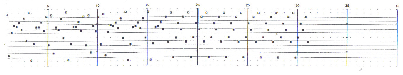
A graphical notation system has been devised to provide a visual reference for the score examples. The coordinate system of the scores is similar to that of traditional musical notation, in that pitch is read on the vertical axis and time is read horizontally. The biggest difference is that the pitch axis of the graphical scores is continuous, rather than discrete, and the distance of a semitone is everywhere the same, rather than variable in size as is the case with traditional notation. This allows an accurate notation of pitch without the use of accidentals, and is as readily adaptable to the notation of infinitely variable pitch as to the equal-tempered scale. For the sake of reference, each score is inscribed with the lines of the traditional grand staff. Dynamic levels in the graphic scores are indicated by the shading of the notes; a very dark note would be quite loud, while a lightly-shaded one is softer. Figure 3 illustrates the notation of a one-octave C major scale, beginning on middle C. The velocity of each note is conveyed by its shading - the darker a note, the louder it is.
It is desirable, in an initial exploration of a potential compositional technique, that highly subjective issues be removed from the picture, or at least minimized as much as possible. The question at hand is not: "How can I make music with this dynamical system?" Rather, it is: "How much music inherently resides in this system?" Once that question is answered, the details of the extraction of the music become the idiosyncratic, personal domain of the composer, and lie outside the domain of this study.
Although many different mappings of chaotic orbits into musical space can be imagined, only one such mapping will be employed for each of the two systems examined in the following chapters. To simplify the presentation and evaluation of the musical product of the chaotic systems in question, the orbits are projected into a uniform pitch space encompassing a four-octave range centered around middle C, in which dynamic levels are allowed to vary between the extremes of loud and soft. Except for the first example from the Lorenz system, the temporal axis (rhythm) is considered non-dimensional and constant.
A graphical notation system has been devised to provide a visual reference for the score examples. The coordinate system of the scores is similar to that of traditional musical notation, in that pitch is read on the vertical axis and time is read horizontally. The biggest difference is that the pitch axis of the graphical scores is continuous, rather than discrete, and the distance of a semitone is everywhere the same, rather than variable in size as is the case with traditional notation. This allows an accurate notation of pitch without the use of accidentals, and is as readily adaptable to the notation of infinitely variable pitch as to the equal-tempered scale. For the sake of reference, each score is inscribed with the lines of the traditional grand staff. Dynamic levels in the graphic scores are indicated by the shading of the notes; a very dark note would be quite loud, while a lightly-shaded one is softer. Figure 3 illustrates the notation of a one-octave C major scale, beginning on middle C. The velocity of each note is conveyed by its shading - the darker a note, the louder it is.
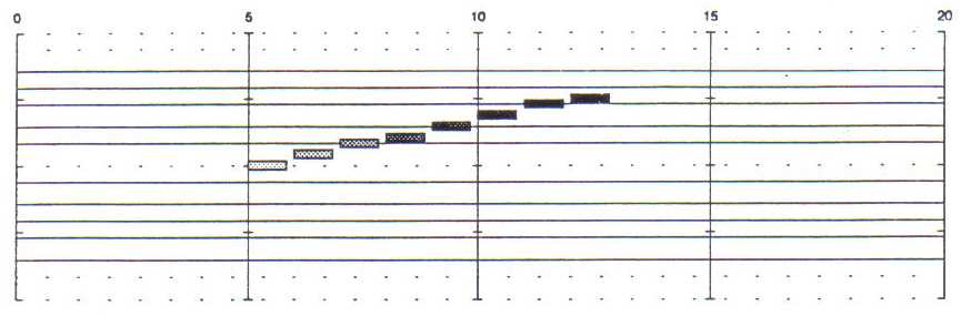
Figure 3: Example of the graphical scoring system. A one-octave C major scale is notated. The scale starts softly and increases in volume. Note that the tick marks on each "bar line" indicate the positions of C's, and that the horizontal dashed lines indicate positions where ledger lines would normally be written. Time is measured in five-second intervals.
The Hénon Map - Technical Description
The Hénon system is a dissipative, two-dimensional iterated map which was first introduced in 1976 by Michel Hénon of the Observatory in Nice19. The Hénon map has no explicit counterpart in the real world, but is an abstract system formulated for the express purpose of studying chaotic systems in general. At the time the map was introduced, most of the known chaotic dynamical systems were defined as continuous flows in three or more dimensions. The computation of numerical solutions to these flows involves the integration of differential equations, a time-consuming and computationally expensive process. The Hénon map, on the other hand, exhibits all of the interesting features of a higher-dimensional chaotic flow (sensitive dependence on initial conditions, interspersed regimes of chaos and periodicity, complex topological structure, a strange attractor, etc.), but is much easier and faster to compute since it is specified in terms of difference equations. In addition, the inaccuracies which arise inevitably in the process of integration may be avoided altogether, rendering the Hénon system more susceptible to mathematical analysis than a higher-dimensional flow.
The Hénon map is expressed by the equations where the succession of points (xo, yo), (x1, yi),(xn, yn) specifies the orbit on the plane, and A and B are constant parameters. The equations are nonlinear by virtue of the squared variable x. In his initial discussion of the system, Hénon assigned the values 1.4 and 0.3 to A and B, respectively; these have since become the "classical" values used to produce the familiar form of the attractor; see Figure 4. A program to generate orbits of the Hénon map in numerical form may be found in Appendix A.2. Hénon's paper, as well as information presented by Thompson and Stewart20, and Fluelle21, provides the substance of the Summary of the behavior of the equations which follow.
Table 4 presents in numerical form the first twenty iterates of the orbit for the parameter values A =1.4 and B = 0.3, from an initial point (0,0). Like the logistic map, the orbit of the Hénon system wanders from point to point along the attractor in an erratic manner.
![]()
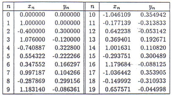
Table 4: Orbit of the Hénon map in numerical form through the first twenty iterates. A=1.4, B=0.3, the initial point is (0,0).
Technically speaking, the attractor itself can never be represented. The points plotted in the three phase portraits of Figure 4 lie on the attractor, but they do not comprise it. (A phase portrait or phase plot is simply a plot of the points along an orbit in the phase space of the system.) Iterates 0 through 3 can still be individually distinguished in Figure 4(c) (the zeroeth iterate lies exactly in the center of the plot), and clearly lie far from the attractor; these points, along with the next two or three, constitute the initial transient portion of the orbit before it settles onto the attractor. There is no specific number of iterates after which one can say that the transient portion has ended and the attractor has been reached. For example, although the fourth iterate can not be individually distinguished in Figure 4(c), at a higher resolution it could be, and would also be seen not to lie on the attractor.
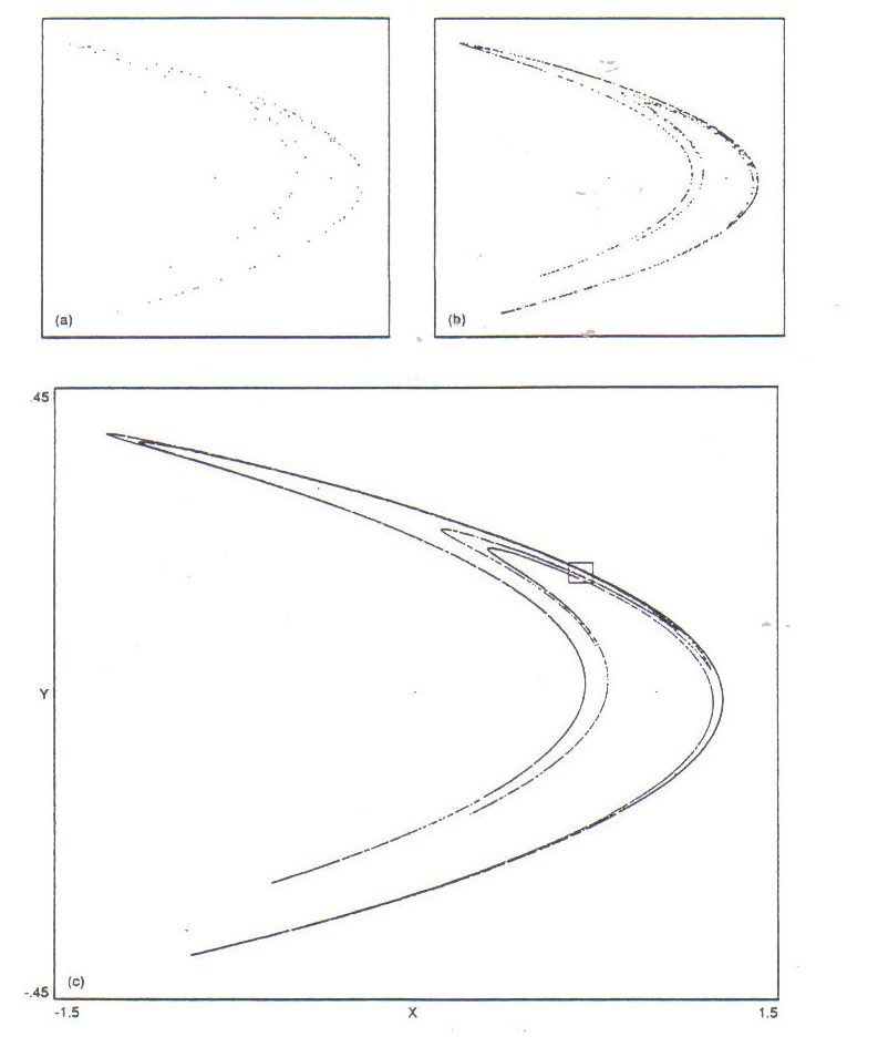
Figure 4: The
Hénon map, (a) after 100 iterations, (b) after
1000 iterations, The Hénon Map after
10,000 iterations. The initial point is
(0,0), the parameters are
A=1.4, B=0.3.
The area of the inset
square is
magnified in Figure 5.
The attractor itself consists of an apparently infinite number of finely spaced filaments, along which the points of a given trajectory are scattered. Figure 5 shows a magnified view of the area within the small inset rectangle in Figure 4(c). The structure of the spacing of the filaments at different levels of magnification is indicative of the fractal Cantor set structure underlying the Hénon attractor. Note that, due to the increasingly small area graphed in the magnification sequence of Figure 5, many more points of the orbit must be computed in order to fill the graphed area to an adequate level.
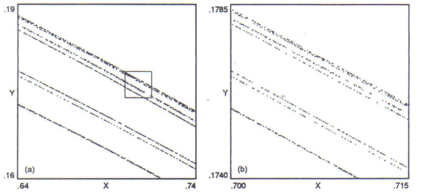
Figure 5: Magnification sequence of the Hénon map. Initial conditions are as for Figure 4. Note that
many more iterations of the map must be computed in order to produce a
sufficient number of points
to fall
within the graphed areas; (a) after 100,000 iterations, (b) after 500,000
iterations.
Figure 6: Basin of attraction of the Hénon map with the attractor superimposed, for parameters A=1.4,B=0.3. Any orbit starting in the shaded areas is repelled from the basin of attraction and tends to infinity.
The basin of attraction is that set of points, any one of which taken as an initial point (x0, y0) of an orbit, produces an orbit which is stable and is drawn to the attractor. Figure 6 shows the basin of attraction as the unshaded area, with the attractor itself superimposed. Points which lie outside the basin of attraction produce orbits which are repelled from this area and escape to infinity.
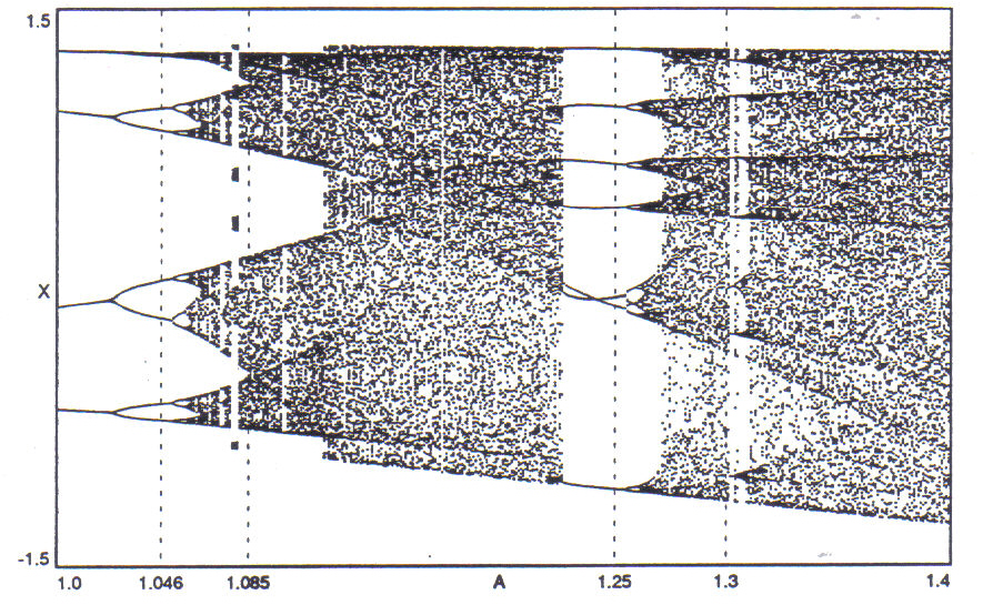
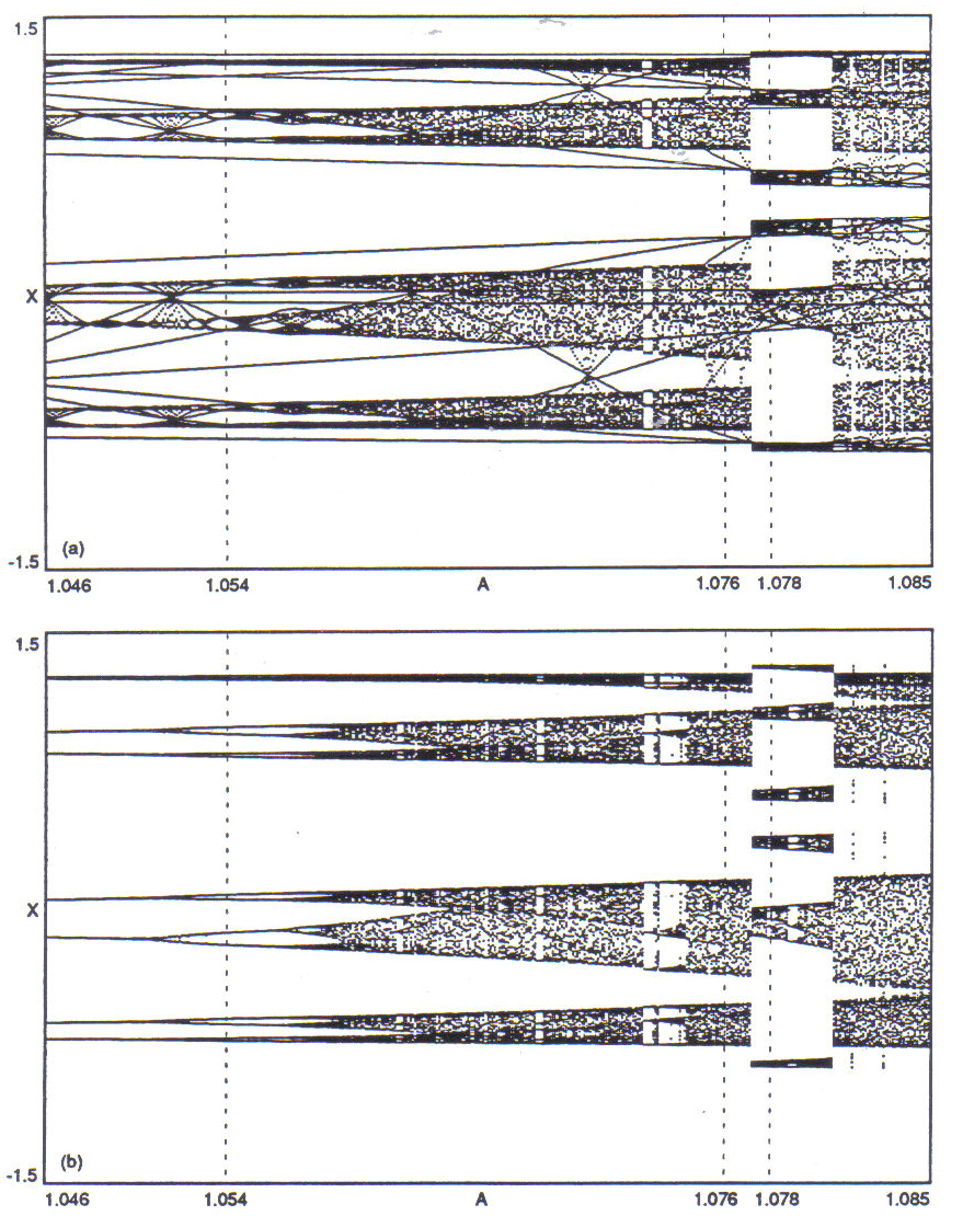
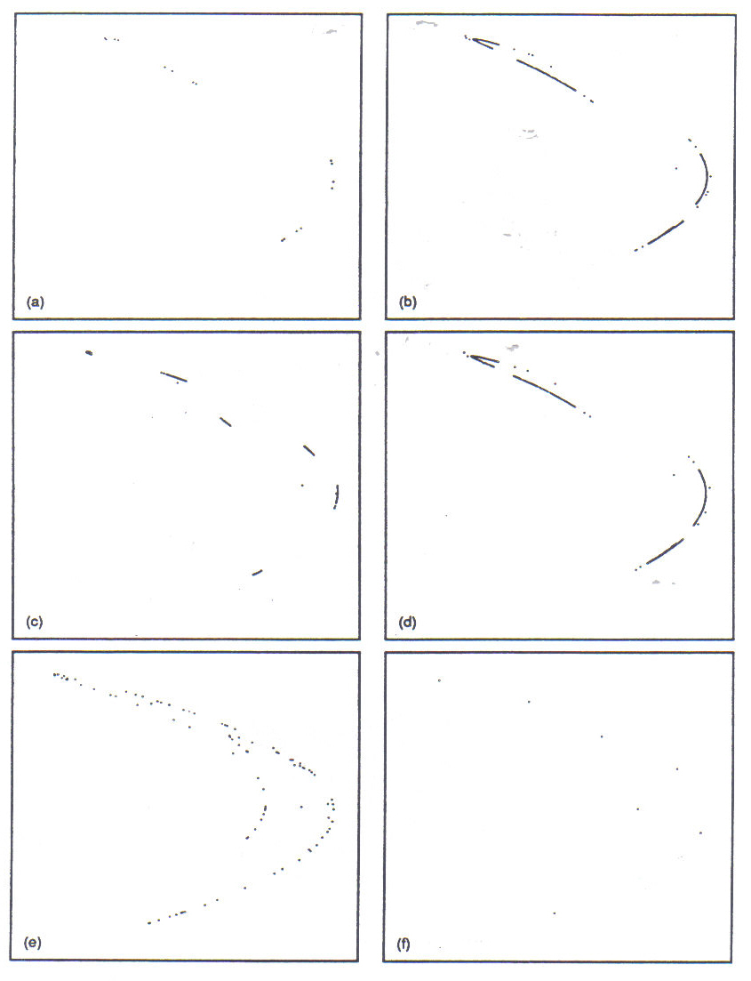
Like the logistic equation, the form of the Hénon attractor varies as the parameter values A and B change. The bifurcation diagrams shown in Figures 7, 8, and 9 exhibit a period-doubling cascade quite similar in form to that of the logistic equation, followed by a regime of chaos interspersed with periodic windows of varying widths. These diagrams were made by holding the parameter B constant at 0.3 and sweeping A across the range of values indicated for each diagram. Phase plots corresponding to some of the values indicated in the diagrams with vertical dotted lines are shown in Figure 10. Note the correspondence, for example, between the four and six-band chaotic regimes located at A =1.076 and A=1.078 in both the bifurcation diagrams and in the two plots of Figures 10(b) and (c). Figures 10(c) and (d) illustrate co-existing attractors for the same value of A emerging from different initial points of the orbit. Other marked positions in the bifurcation diagrams correspond to orbits chosen for the musical examples following in the next section.
Figure 7a: (a) Bifurcation diagram of the Hénon map, initial transient behavior (the first 150 iterations)
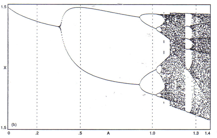
Figure 7b: settled, stable behavior (the next 150 iterations). Each plot sweeps parameter A from 0 to 1.4, holding B constant at 0.3. The initial point of all orbits is the origin, (0,0).
Figure 8: Magnification of a section of the bifurcation diagram from A.1 to A.1.4. A period 16 bifurcation is discernible just before the onset of the chaotic regime at approximately A=1.055. Note the large period 7 window around A.1.25, as well as other, less extensive regimes of periodicity interspersed through the chaotic regime. This diagram shows the settled behavior of the system.
Figure 9: Further magnification of the Hénon bifurcation diagram, focusing on the transition to turbulence. The two illustrations plot (a) transient behavior (the first 150 iterations) b) settled behavior (the next 150 iterations). At this level of resolution, an additional period 32 bifurcation can be barely discerned just above A=1.054. Note as well the abrupt shift in the structure of the attractor, from four bands of chaos to six, which occurs between A.1.076 and A.1.078.
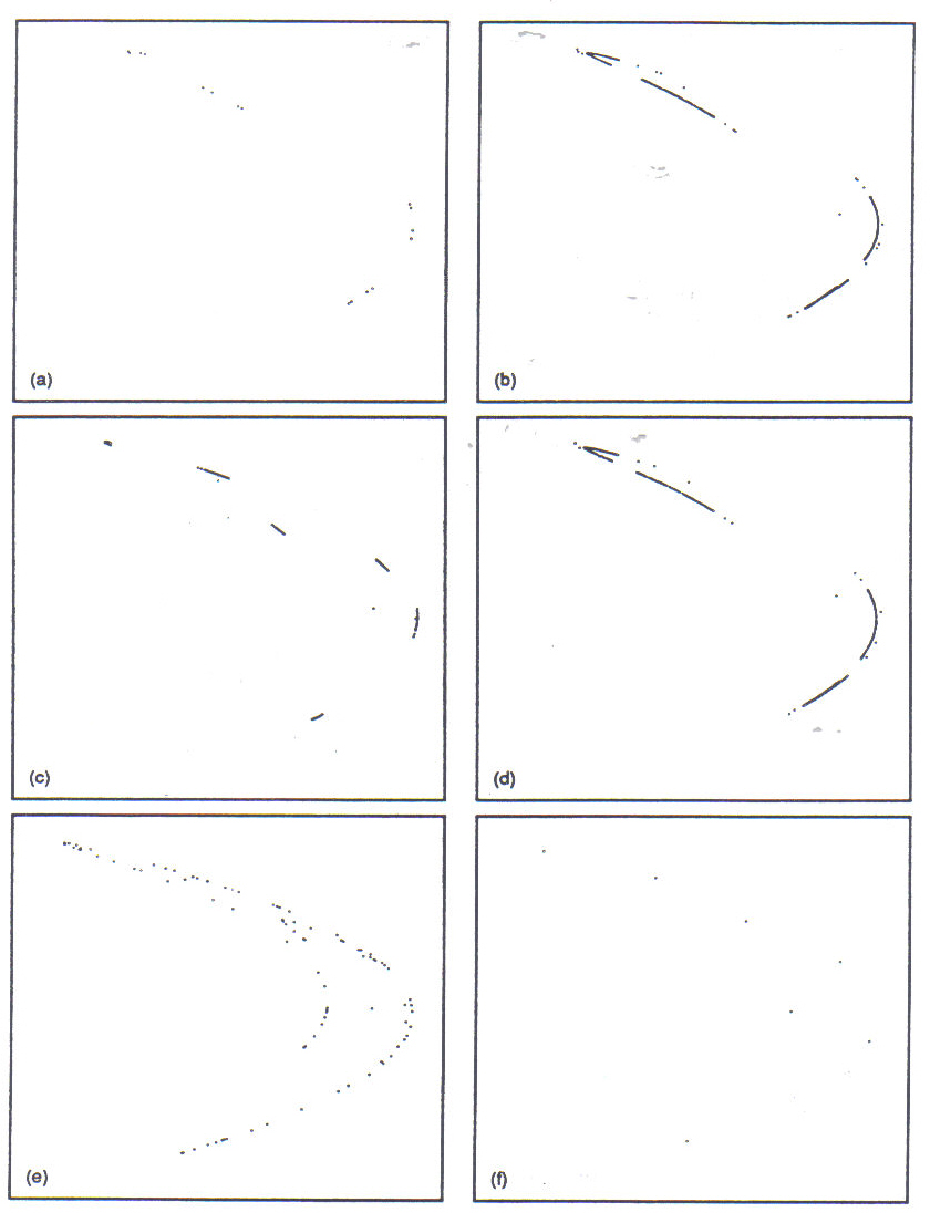
Figure 10: Phase portraits of the Hénon map. Parameter B=0.3 for all orbits. Initial point is the origin (0,0) for all orbits except (d); (a) period 16 orbit at A=1.054, (b) chaotic attractor at A=1.076, (c) chaotic attractor at A=1.078, (d) co-existing chaotic attractor at A=1.078, from initial point (.1, 0), (e) first 150 iterations of apparently chaotic orbit at A=1.3, however, (f) period 7 orbit emerges from chaos after approximately 120 iterations at A=1.3.
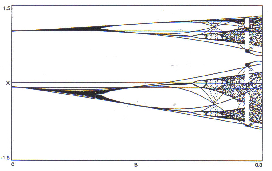
Figure 11: Bifurcation diagram of the Hénon attractor plotting B against x. Parameter A is constant at 1.1 for all trials. The first 150 points of each orbit are plotted.
For the sake of comparison, a bifurcation diagram sweeping the parameter B and holding A constant is shown in Figure 11. Bifurcation diagrams plotting changes in y may be produced as well, and are similar in appearance to those plotted against x, except for the change in scale. The behavior of both variables is globally similar: if x is periodic, y is also periodic, if x varies chaotically, so does y.
Further discussion on the Hénon map may be found in Shaw, Eckmann and Ruelle23t, Ruelle24, and Froehling, et al..25.
Musical Examples
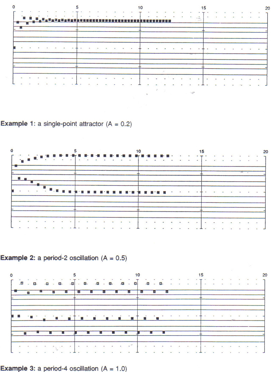
Musical mappings of the Hénon system exploring a range of characteristic behaviors were made over 9 different values of the parameter A. These values, 0.2, 0.5, 1.0, 1.046, 1.054, 1.076, 1.078, 1.3, and 1.4, may all be located among the phase plots and bifurcation diagrams in the preceding section. The initial point (0,0) is used for all examples (Example 10 excepted), and the parameter B is held constant at 0.3 throughout.
There are a large number - infinite, actually - of possible mappings of the phase space to the musical domain. Each of the variables x and y could be mapped to any musical parameter; in addition, a variety of orientations are possible. For example, values along each axis could be mapped inversely to a given parameter, such that an increase in the value along the axis would cause a decrease in the value of the musical parameter. The phase space could be quantized, interpreted logarithmically, or multiplied. Clearly a comprehensive exploration of possible mapping configuration would take several lifetimes.
For simplicity and the sake of space, only one mapping configuration is used in the examples included in Appendix A. This configuration maps values along the y-axis to pitch, and values along the x-axis to dynamic level. In all of the examples, the extent of the Cartesian phase is taken to be -1.43 to 1.43 on the x-axis, and -0.43 to 0.43 on the y-axis. These values were discovered empirically to encompass the totality of the phase space of the Hénon map under the conditions employed in the musical examples.
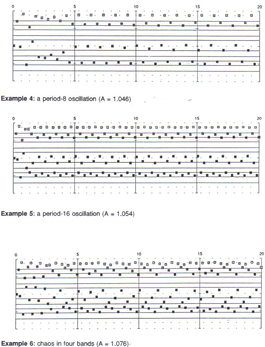
The first examples are straightforward and require little explanation or comment. Example 1 begins with an oscillation between two values which, during a brief transient phase, is quickly damped to a single point, a sequence of repeated notes. In Example 2, the transient phase consists of a widening oscillation which stabilizes on a period-2 attractor. In Example 3, the transient portion of the sequence appears shorter at first glance than it does in Examples 1 and 2, but in fact it is just about as long, requiring 16 iterations before it stabilizes. In Example 4, the transient portion is both longer and more irregular than in the previous examples. The period-8 orbit is finally stabilized after twelve seconds. Example 5 illustrates a period-16 oscillation following a short transient phase.
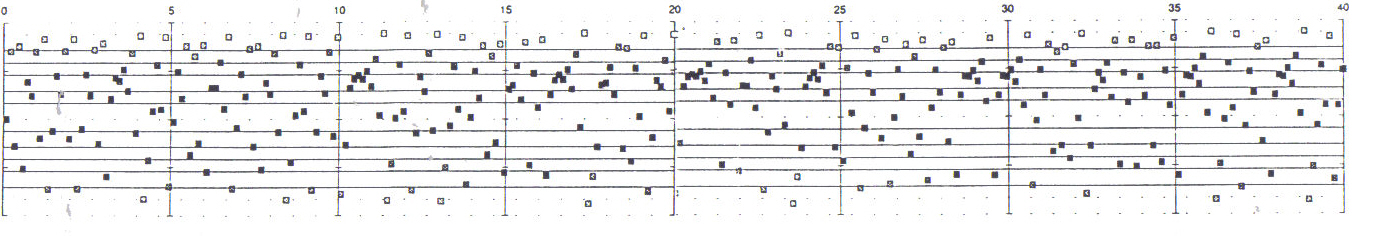
Example 6 is taken from a regime in which the phase space is divided into four distinct bands of chaos. Two broad layers are easily perceived, each of which is in turn subdivided into two bands. In the lowest band of the lowest layer, extending from approximately B--D# in the octave below middle C, a downward-tending three-note pattern is apparent as the primary constituent, which is interspersed with a longer pattern of either four or five notes. The second band, extending from approximately the F# below middle C to the D above, is similar to the first band, but with a contrary sense of motion. In the upper layer, the third band, from the C an octave above middle C to the F# above that, is similar to the lowest band, but with a slightly wider ambitus. The fourth and highest band is also like the first and third, but compressed in ambitus and offset in phase slightly.
Although it appears quite periodic, six distinct chaotic bands mark the texture of Example 7. The effect is of greater regularity or periodicity than in Example 6, because of the reduced range in which the values of each band may vary. Examples 6 and 7 are illustrations of what might be called "noisy periodicity." Example 8 illustrates an interesting sequence in which a long transient phase eventually settles into a period 7 orbit.
Example 9 is generated from the full-blown chaotic attractor plotted in Figure 4. Note that the louder notes are clustered in the middle of the range, corresponding to middle portion of the boomerang-shaped attractor. A clearly audible complex hocketing effect may be discerned from sonic realizations of this texture as the ear forms independent melodic lines from notes of similar velocity levels arrayed within consistent registral dispositions.
Example 10 is an example of sensitive dependence on initial conditions as applied to the generation of harmony. Three voices are generated synchronously, which proceed from initial points which are very close together: (0.000000, 0), (0.000001, 0), and (0.000002, 0). The three voices/orbits remain virtually identical through at least twenty iterations before the effect of their different initial positions precipitates a rapid divergence of the orbits from one another. Note that the first voice in this example (the one which begins exactly at the origin) is identical with the sequence in Example 9, with the reduced tempo taken into account.
The Lorenz System - Technical Description
The earliest explicit recognition that stable regimes of chaotic behavior could arise spontaneously from the dynamics of a set of nonlinear equations is generally attributed to the mathematician and meteorologist Edward Lorenz in a landmark 1963 paper entitled "Deterministic nonperiodic flow"26. From a conventional model of the dynamics of fluid convection, Lorenz evolved a simplified version expressed as a system of three partial differential equations,
x - σ(y-x)
y = Rx- y -yx
z = xy = Bz
where, R and B are positive constant parameters. The system becomes unstable if any of these parameters are negative. The equations are nonlinear by virtue of the multiplication of the variable x with each of the other two variables of the system. Solutions to the equations may be described as a continuous trajectory or a flow embedded in a three-dimensional Euclidian space. The equations specify a dissipative system whose basin of attraction encompasses all of real space. The clear exhibition of extreme sensitivity to initial conditions that Lorenz was able to demonstrate in the behavior of this system had profoundly negative implications for the feasibility of long-term weather prediction. Since, by definition, an accurate measurement of the instantaneous state of the atmosphere is impossible (because of the finite resolution of measuring devices), then the long-term predictions of any computer simulation used to model atmospheric conditions forward from the present state will eventually diverge exponentially from the actual conditions. This situation has come to be known as the "butterfly effect," because of the implication that a phenomenon as seemingly insignificant as the flutter of a butterfly's wings in Japan may exert an enormous influence on the weather in California a week later.
Lorenz adopted the parameter values 6 = 10, R = 28 and B = 8/3 in his numerical study of the equations. These values reveal a chaotic attractor bounded within a region of space whose extent is a function of the three constant parameters. The orbit along the attractor describes an alternating sequence of spiral revolutions around two stationary points, P1 and P2, located at (1√(B (R - 1)), √(B(R - 1)), (R - 1)) and (-√((B(R - 1)}, -i√(B(R -1)), (R - 1)); see Figures 12 and 13. A typical orbit spirals out from one of the stationary points a variable number of times (as few as one, or as many as 50 or more revolutions) until it is attracted towards the neighborhood of the other stationary point, and begins the cycle again.
Like the logistic equation and the Hénon map, the Lorenz system exhibits regimes of single-point attraction, periodicity, and chaos. The creation of bifurcation diagrams for the Lorenz system, however, is extraordinarily more expensive and time-consuming to compute due to the fact that the equations must be integrated over extended spans of time in order for the underlying order to become apparent. In his extensive survey of the system, Sparrow27 provides several hand-drawn sketches of the locations of some of the bifurcation nodes in the total phase space. It is from Sparrow's study that the following summary of the global behavior of the system is condensed.
A third stationary point (in addition to P1 and P2) exists at the origin (0, 0, 0), and is stable for all parameter values -meaning that any orbit which begins there, stays there. The origin is also globally attracting for 0 < R < 1 meaning that all orbits tend toward the origin and remain there if R < 1, no matter where they are initiated.
The z-axis is invariant for all parameter values. Any orbit which starts on the z-axis (the line in the phase space along which both x and y are 0) will remain on that axis and tend toward the origin.
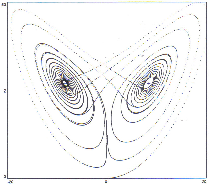
Figure 12: Phase portrait of the Lorenz system projected onto the (x,z) plane along the y-axis. The attractor lies within a region of real space measured in the positive direction along the z-axis. The crosshairs at the centers of the two lobes mark the locations of the two stationary points P1 and P2. Constant parameters are a = 10, R = 28, B = 8/3. The initial point is (.1, .1, .1), located at the bottom of the graph right above the "X".
Figure 13: Phase portraits of the Lorenz system projected onto (a) the (x,y) plane, and (b) the (y,z) plane. Crosshairs mark the locations of the stationary points. Parameters values and initial point are the same as for Figure 12. Both graphs plot the same orbit.
The critical value R - 24.74 marks a reversal in the character of the two stationary points P1 and P2. At the supercritical value adopted by Lorenz, R 28, these two points are non-stable or repelling, whereas at subcritical values of R, they are stable or attracting. In other words, for subcritical values of R, all orbits are attracted to one of the stationary points P1 or P2, or to the origin. Orbits are not necessarily chaotic for all super-critical values of R, however. Regimes of periodicity are interspersed within regimes of chaos across a wide range of values. Figure 14 (a) illustrates a periodic orbit at R = 150. A change in the value of parameter B to 0.25, however, while leaving R at 150, produces another chaotic orbit; see Figure 14(b).
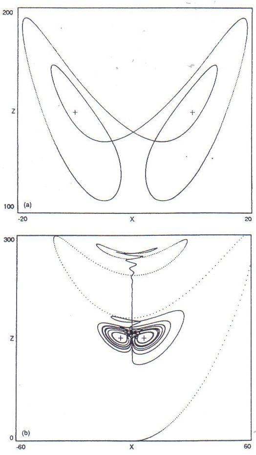
Figure 14: Two orbits of the Lorenz attractor at
R = 150,
sigma
= 10;
(a) periodic
orbit for B=8/3,
shown
without the initial transient; (b) chaotic orbit for
B=1/4,
including the
transient portion. Both
portraits are projections onto the (x,z)
plane along the y-axis, and the initial point is also (.1, .1, .1) for
both. Crosshairs mark the locations of the stationary points P1 and P2.
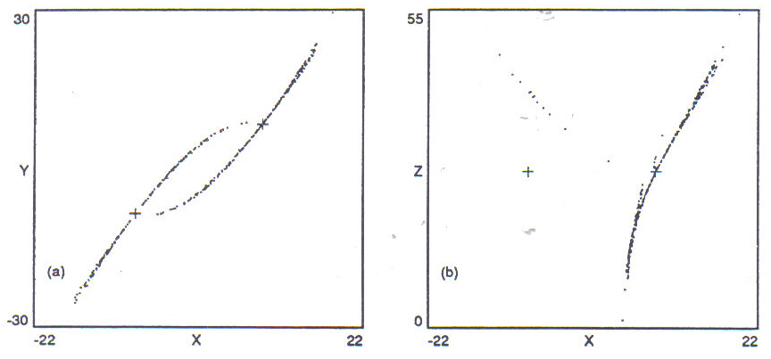
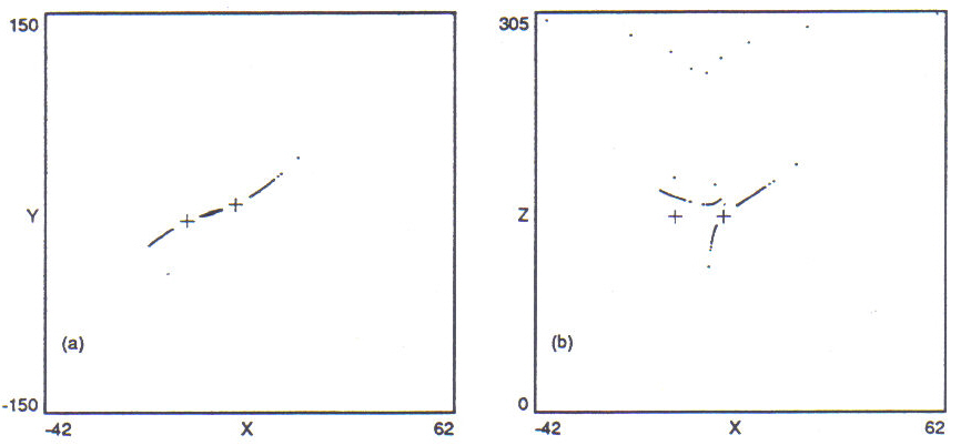
An alternate perspective on the structure of continuous dynamical systems is afforded by the surface of section obtained by plotting the intersection of the orbit with a plane which slices through its phase space. The resulting two-dimensional map plots the position of the trajectory as it "punctures" the plane of the section. A method of analysis of dynamical systems based on this procedure was developed by Poincaré toward the end of the nineteenth century. Also called Poincaré sections or return maps, these two-dimensional reductions of the dynamics of a higher-dimensional flow bear a strong resemblance to iterated maps such as the Hénon system. For example, a Poincaré section of a periodic orbit would show simply as a few points on the plane, similar to phase plots of periodic regimes of the Hénon map. For a chaotic orbit, a scattering of points across the plane is produced. Figures 15 and 16 illustrate surfaces of section taken across planes which pass through one or both of the stationary points P1 and P2. These sections correspond to the parameter values and initial conditions plotted in Figures 12 and 14(b). Figure 16, especially, illustrates the reduction of phase-space as the orbit passes through its transient phase and into the region of the attractor in the center of the plot.
Despite the data reduction represented in a Poincaré section, its computation requires as much time as the computation of the entire trajectory does, because it is still necessary to compute all of the points along the orbit between punctures of the sectional plane in order to know where the next puncture will be. The derivation of a set of difference equations (an iterated map) from a given set of differential equations (a continuous flow), in a manner which would allow a direct computation of the Poincaré section of the flow, is unfortunately neither trivial nor obvious. There is some speculation that a higher-dimensional flow exists for every true iterated map (of which the map might be considered the surface of section of the hypothetical flow), but the existence of such has not been demonstrated to date. Nonetheless, Shaw28 demonstrates morphological similarities between the Hénon attractor and the hypothetical section of a certain generic flow.
Further discussion on the Lorenz equations may be found in Thompson and Stewart 29, Lichtenberg and Lieberman30,Helleman31,Ruelle32, and Farmer et al.33.
![]()
![]()
Figure 15: Surfaces of section through the Lorenz attractor, for the parameter values sigma = 10, R = 28, and B = 8/3;(a) on the (x,y) plane at z=(R-1)=27, (b) on the (x,z) plane at y = 8.485281. Crosshairs mark the locations of the stationary points.
Figure 16: Surfaces of section through the Lorenz attractor, parameter values sigma = 10, R = 150, and B = 1/4; (a) on the (x,y) plane at
z=(R-1)=149, (b) on the (x,z) plane at y = 6.103278. Crosshairs mark the locations of the stationary points.
Musical Examples
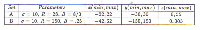
Musical mappings of orbits of the Lorenz equations were made with the two sets of parameters explored in the preceding technical section, namely sigma = 10, R = 28, B =8/3 (Set A), and sigma=10, R = 150, B 1/4 (Set B). Because of the different region of phase space occupied by the orbit under each of these two sets of parameters values, the ranges along each of the three axes of the coordinate space which map to minimum and maximum values of the musical domain space are different as well. These relationships are summarized in Table 5. The first example (of Appendix B) explores the musical potential of the Lorenz equations as a continuous flow, while examples 2 through 5 map surfaces of section into the musical domain. Except for the second voice in the first example, the initial point of each sequence is (.1, .1, .1).
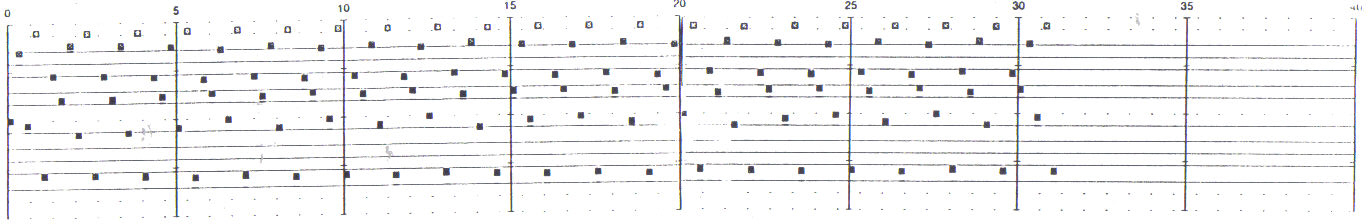
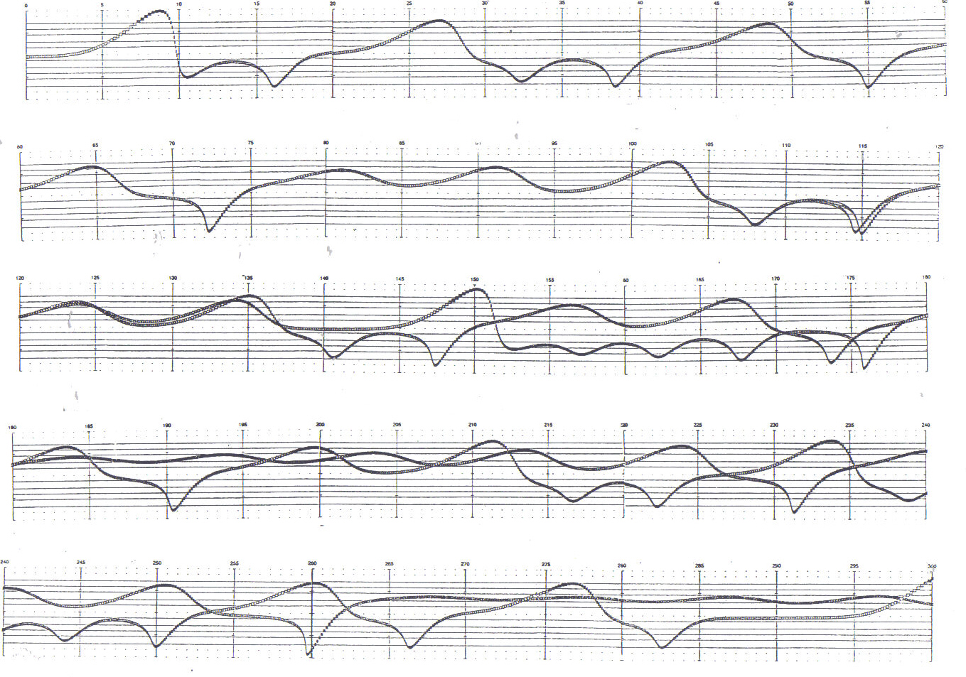
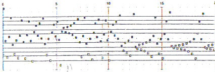
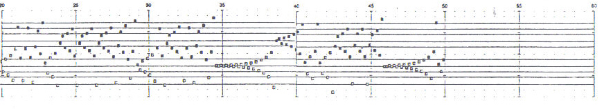
Example 1 charts the courses of two orbits which begin at almost the same location, specifically (.1, .1, .1) and (.1001, .1001, .1001). The two orbits remain virtually identical for at least 100 seconds before the difference in their initial positions causes them to diverge. This example lasts just over five minutes, a span barely long enough for the initial transients to subside and for behavior more typical of the settled orbit to manifest itself. Pitch varies according to z, velocity according to x, and the inter-note onset time according to y. A given mapping configuration has the effect of aligning parameters into consistent relationships: for example, around middle C notes are all at a medium velocity and speed, while the lowest notes are also the loudest and fastest, etc. The low, fast dips correspond to single revolutions of the orbit around the stationary point located in the (-x, -y, z) quadrant. On the grand staff, this point is located at approximately the F below middle C. The "humps" in the upper register correspond to revolutions around the other stationary point, in the (x, y, z) quadrant. This point is located at approximately G above middle C. Although the orbit makes only single and double revolutions around the stationary points at the beginning, this behavior is only transitory. A sequence of five revolutions around the lower stationary point begins after 150 seconds (note the dips located approximately at 152, 157, 162, 168 and 176 seconds), and a similar sequence around the upper stationary point begins after 180 seconds. The outward spiral of the orbit as it is repelled from a stationary point is reflected in the increasing ambitus of the oscillations in each of these sequences. The last revolution before a transition to the opposite stationary point is always the greatest in extent.
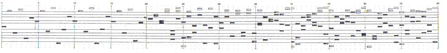
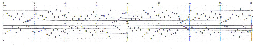
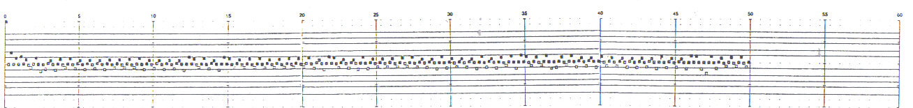
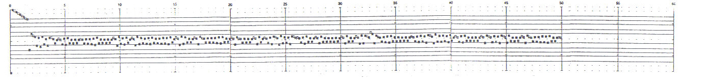
Example 2 is made from a Poincaré section taken on the plane at z = R-1 = 27 (see Figure 15(a)), which includes both of the stationary points P1 and P2. In the graphical score, these two points are located at the vertices of the sideways V-shaped figures visible throughout the examples. These figures, opening to the right as time moves forward, are evidence of the outward spiral of the orbit around each point. The orbital information which is represented over a span of five minutes in Example 1 occupies only the first ten seconds of Example 2. These examples thus present in a condensed format a picture of the behavior of the Lorenz system over a much longer span of time. As with the continuous flow in Example 1, the mapping aligns musical parameters in a consistent manner: all of the notes in the lower part of the range (around the lower stationary point) are softer than those in the upper part of the range. Example 3 is a section taken at y =.413(R-1)) = 8.485282. Although this example is made from precisely the same orbit as that of example 2, the pattern recorded is entirely different due to change in the geometry of the sectional plane with respect to the course of the flow.
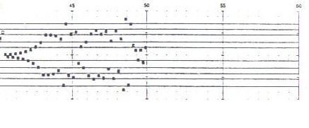
Example 4 is made from a section at z = 149 (= R - 1) using the parameters of Set B; see Figure 16(a)). The drastic reduction in the range of the musical texture as the initial transient dies out in the first several seconds is a demonstration of the loss of energy common to all dissipative systems. The nature of the attractor visible in the center of the pitch range is also clearly quite different from that of examples 2 and 3, even considering the change of scale. Example 5 is made from a section at y 14B(R-1)} = 6.103278 (see Figure 16(b)). Interestingly, irregularities in the texture occur here at locations where the corresponding texture in Example 5 is fairly smooth. Like Examples 2 and 3, these sections demonstrate the variation in textural contour which can be attained by judicious placement of the sectioning plane.
Table 5: Parameters and coordinate space mappings
Musical Implications
In a discussion concerning historical changes in the structure of musical forms which have been brought about by changes in the nature of local structures, Boulez begins with a quotation from Claude Levi-Strauss:
Form and content are of the same nature and amenable to the same analysis. Content derives its reality from its structure, and what is called form is the "structuring" of local structures, which are called content.34
Boulez goes on to say:
We have seen that the generation of networks of possibilities, which are the raw material for Popérateur -to use a significant term of Mallarmé' - has from the outset tended increasingly to produce a material that is constantly evolving. [W]e can only work towards connections that are constantly evolving, and in the same way this morphology will be matched by a correspondingly non-fixed syntax.35
Although that was written well before
the subject of chaos burst onto the international
scene, Boulez' thoughts dovetail
very nicely with the quality of material that one can expect
to generate as a matter of course by means of nonlinear dynamical systems such
as those![]() discussed in this work. The subject matter of chaotic systems is, indeed, the
structuring of
local
structures, in connections that are constantly evolving.
discussed in this work. The subject matter of chaotic systems is, indeed, the
structuring of
local
structures, in connections that are constantly evolving.
Nonetheless, there is a quality to the music of chaos which is distinct and not to be confused with products of the human mind -although there is also an undeniably natural feel to much of the material produced by the methods explored in this work. Still, the quality of these materials is closer to that of figuration than to bel canto aria. If music may be thought of as the art of projecting, in an interesting way, a moving line or a group of moving lines through a multi-dimensional grid measured in terms of frequency, volume, time and timbre (which is itself multi-dimensional), then nonlinear dynamical systems furnish a powerful and novel means for the specification and control of these lines through such a grid space. The process of understanding these systems is the process of learning how they behave under a variety of conditions. Their global behaviors are learnable and therefore predictable from the point of view of being useful in the generation of musical raw materials. Orbits which are known to produce desirable effects may be calculated on demand. One may treat these systems as musical commodities, natural resources to be exploited at will. In fact, the term "natural resource" is doubly meaningful because of its dual associations: textures generated from these systems are "natural" in that they undeniably share qualities of real-world phenomena to which we are able to respond. Textures generated from these systems are also "resources" in that they may be exploited (or not) like any other musical resource.
There remains much room for experimentation with more complex mapping schemes not explored in this study. For example, the succession of (x,y) coordinate pairs in orbits of the Hénon system need not be consistently mapped to an invariant set of musical parameters throughout the course of a sequence, but may alternate between two complementary mappings; e.g., (x0,y0) to (frequency, amplitude), (x1,y1) to (frequency, amplitude), (x2,y2) back to (frequency, amplitude), and so on. This produces a new musical texture quite different from those presented in the earlier examples generated from the Hénon map, but which still contains essential qualities of that system. Orbital mappings may be quantized on the computer to any degree, in any dimension: pitch, time, volume, timbre. Additionally, the output of one system may be coupled to the input of another system, and chaotic sequences may be used to drive production grammars in place of white or colored noises which are often used. Nor need the utility of these systems be confined to the generation of note textures. The Lorenz attractor, for example, might be quite interesting as a three-dimensional spatialization path, or in a waveform synthesis algorithm.
A number of interesting qualities are exhibited in chaotically produced textures. The paradoxical condition of a "consistent variety" of motivic material generated is foremost among them. The materials carry with them an inherent suggestion that they be employed in sequences of (at least) intermediate duration, because the character of the material is made manifest only after a number of iterations. While the overall behavior of a given chaotic orbit is, in a strict sense, not predictable, in an operational sense, it is. It is clear, for example, that the settled orbit of the Hénon map will not suddenly visit a point far from the attractor, or that a periodic oscillation will suddenly come to an end and turn chaotic. Nonetheless, these systems are productive of sequences of events in which sudden, unexpected changes may occur - albeit within the limits of their global repertoire of behavioral possibilities. This is a type of bahavior not seen in purely random
sequences, which maintain an even consistency throughout, incapable of evoking surprise. Spectra of chaotic systems do, however, resemble 1/f noise in that longer-term correlations are present and obvious (see Farmer, et al.36). Nonetheless, the character is noticeably different. Chaos is generated by deterministic procedures (there is therefore a presence of some measure of "volition," even if it is only exercised by mindless equations), whereas white noise and 1 /f-noise are probabilistic outcomes.
These qualities notwithstanding, the long-term behavior of all of these systems is static. The equations contain no inherent specifications of drive or impetuousness. There is no overarching teleological force guiding the sequence of notes to some grand conclusion. There is no phrase structure. What is missing in these materials is directionality, the sense that the structure evolves according to the dictates of a human will. All of these qualities must be added by the musician "by hand." Moments of localized directionality, in which a serendipitous turns of events catches the attention, must be isolated and elaborated.
Nonlinear dynamical systems have the potential for creating the theoretical foundation of a new and idiosyncratic idiom of computer music, of an intrinsic fluency wholly independent of external derivations from tape and instrumental music. Chaotic systems are a means by which computer music may move beyond the limited possibilities of sequencing (a technique appropriated from analogue electronic music) or the role of sound processor to which it is often consigned. Dynamical systems are versatile generators of "meta-sequences" - sequences of motivic material made more flexible by virtue of their specification as rules of natural behavior rather than as fixed sets of notes. Chaos affords composers working with computers the opportunity to address musical issues at a level of organization which has remained largely uninvestigated in the medium to date: the generation of melodic and harmonic materials at the note level.
Appendix A - Score Examples
Example 7: chaos in six bands (A - 1.078)
Example 8: period-7 oscillation afater and extended transient (A- 1.3)
Example 9: chaos (A - 1.4)
Example 10:chaos, illustrating sensitive dependence on initial conditions
Example 11: two voices divergin due to sensitive dependence on initial conditions
Example 12: section at z= 27
Example 13: section at y - 8.4852828
Example 14: section at z - 149
Example 15: section at y - 6.103278
1 This paper is excerpted
from the author's dissertation of the same title (UCSD, 1990). Reproduced here
are portions of chapters 1, 2, 3, and 6.
2 Luchini, P.
"On a singularity encountered during the numerical study of a
fluid-dynamics boundary-layer problem." In Pnevmatikos,
Bountis and Pnevmatikos, eds.,
International Conference
on Singular
Behavior and Nonlinear Dynamics, vol. 2, pg. 581-600, World
Scientific, Singapore, 1989.
3 Treve, Yvain M. "Theory of chaotic motion with application to controlled fusion research." In Siebe Jorna, editor, Topics in Nonlinear Dynamics: A Tribute to Sir Edward Bullard. AIP Conference Proceedings, No. 46, pg. 147-200, American Institute of Physics, New York, 1978.
4
West, Bruce. "Fractal
physiology; a
paradigm for adaptive response." In Prevmatikos, Bountis and Pnevmatikos, eds.,
International Conference on Singular Behavior and Nonlinear Dynamics, Vol.2,
pg. 643-664, World Scientific, Singapore, 1989.
5
Davydov, A.S. "High temperature supercondictivity in ceramic
compounds and bisoliton
model." In Pnevmatikos,
Bountis and Pnevmatikos, eds., International Conference on Singular Behavior
and Nonlinear Dynamics, Vol.2, pg. 327-341, World Scientific, Singapore,
1989.
6 Wunderlich W., Stein E.
and Bathe, E.-J., eds. Nonlinear Finite Element Analysis in Structural
Mechanics, Springer-Verlag, Berlin, 1981.
7 Moser, J. "Is the System Stable?"
The Mathematical Intelligencer, 1:65-71, 1978.
8
May,
Robert
M. "Nonlinear problems in ecology and resource management," In loos,
Heileman, and Stora, eds.,
Comportment
chaotique des systèmes determinantes,
pg.
513-564,
North Holland Publishing Co., Amsterdam, 1983.
9 Gleick, James. Chaos: Making a New Science. Viking Press, New York, 1987.
10 Mandlebrot, Benoit. The Fractal Geometry of Nature. W.H. Freeman, New York, 1983.
11 Goldberger, Ary L, Rigney, David R., and West, Bruce, J. "Chaos and fractals in human physiology." Scientific American, 262(2): 42-49, February 1990.
12 Peitgen, Heinz-Otto and Saupe, Dietmar. eds. The Science of Fractal Images. SpringerVerlag, New York, 1988.
13
op.cit.
pg. 231.
14 May, Robert, M. "Simple mathematical models with very complicated dynamics." Nature, 261:459-457, June 10, 1976.
15 Thompson, J.M.T. and Stewart, H.B. Non-Linear Dynamics and Chaos. John Wiley and Sons, Chichester, 1986.
16 Ruelle, David. "Dynamical systems with turbulent behavior." In Dell'Antonio, Doplicher, and Jona-Lasinio, Eds. international Conference on the mathematical problems and theoretical physics. Lecture Notes in Physics, Volume 80: Mathematical Problems in Theoretical Physics, Springer-Verlag, Berlin, 1978, pg. 341-360.
17 Devany, Robert L. An Introduction to Chaotic Dynamic Systems. Addison-Wessley, Redwood City, California, 1987.
18 Moon, Francis, C. Chaotic Vibrations: An Introduction for Applied Scientists and Engineers. John Wiley and Sons, New York, 1987.
19 Henan, Michel. "A two-dimensional mapping with a strange attractor." Communications in Mathematical Physics, 50: 69-77, 1976.
20 op.cit.
21 Ruelle, David. "Strange Attractors," The Mathematical Intelligencer, 2:126-137, 1980.
![]() 22
Shaw, Robert. "Strange attractors, chaotic behavior, and information flow,"
Zeitshrift Mir
NaturfOrshung,
36a: 80-112,1981.
22
Shaw, Robert. "Strange attractors, chaotic behavior, and information flow,"
Zeitshrift Mir
NaturfOrshung,
36a: 80-112,1981.
23 Eckmann, J.-P., and Ruelle, David. "Ergodic theory of chaos and strange attractors." Review of Modem Physics, 57(3):617-656, 1985.
24 Ruelle, David. "Dynamical systems with turbulent behavior." in Dell'Antonio, Doplicher, and Jona-Lasinio, eds. international Conference on the mathematical problems in theoretical physics. Lecture Notes in Physics, Volume 80; Mathematical Problems in Theoretical Physics, pages 341-360; Springer-Verlag, Berlin, 1978.
25 Froeling, Harold, Crutchfield, James P., Farmer, Doyne, Packard, Norman H., and Shaw, Robert. "On determining the dimension of chaotic flows." Physics, 3D:601-617,1981.
26 Lorenz, Edward N. "Deterministic nonperiodic flow," Journal of the Atmospheric Sciences, 120:120-139-141. 1963.
27 Sparrow, Colin. Ther Lorenz Euqations, Bifurcation Chaos and Strange Attractors, Applied Mathematical Sciences, Volume 41, Springer-Verlang, New York, 1982.
28 op.cit.
29 op.cit.
30 Lichtenbuer, A.J. and Lieberman, M.A. Regular and Stochastic Motion. Applied Mathematical Sciences, Volume 38, Springer-Verlag, New York, 1983.
31 Hellerman, Robert H.G. "Self-generated chaotic behavior in nonlinear mechanics." In Fundamental Problems in Statistical Mechanics V, pg. 165-233, North-Holland Publishing Company, Amsterdam, 1980.
32 Ruelle, David. "Strange Attractors." The Mathematical intelligencer, 2:126-137,1980.
33
Farmer, Doyne; Crutchfield, James P.; Froehling, Harold; Packard, Norman, H.
and Shaw,
Robert. "Power Spectra and mixing properties of strange attractors." In Robert
H. G. Hellemen, ed.
Nonlinear Dynamics,
International
Conference on Nonlinear Dynamics. Annals of the New York
34 Boulez, P. Orientations, Harvard University Press, Cambridge, Massachusetts, 1985, trans. by Martin Cooper, pg.90.
35 ibid. pg.90
36 op.cit.